Animation Exercise — Tangents
1. Set your project to understanding_maya\Chapter03\Animation_tangents.
2. Open the scene animation_tangent_spheres.ma.
3. You’ll see a sphere sitting on the ground. Make sure your animation playback preferences have been set to real-time (24 fps). Press play. The sphere goes up and down over the course of two seconds. Notice how the sphere’s motion is abrupt and mechanical. When the animation is played, the sphere goes from stillness to full speed in an instant, and when it changes directions it does so suddenly. Select the sphereLinear object and then move the cursor over the Graph Editor panel and press the a hotkey. You will see a function curve that describes the sphere’s motion. The three points represent keys; the curve represents the in-between frames (also called interpolation).
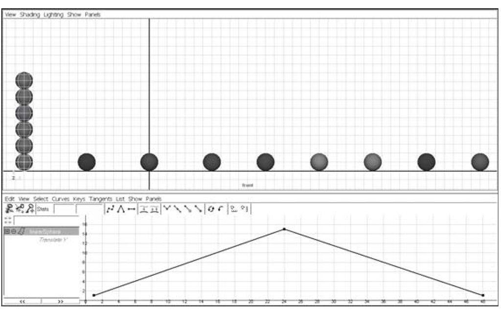
4. Go ahead and play the animation again with the sphereLinear object selected. Notice the function curve in the Graph Editor as the sphere goes up and down (see Figure 3.40). See how the abrupt change in direction on frame 24 matches the shape of the curve? The Graph Editor is simply a plot of a key’s value (the vertical ruler on the left) over time (the horizontal ruler on the bottom). If you were to draw a line straight up from frame 24 until you hit your curve and then draw a line to the left until you hit the value ruler you would find a value of 12 units up on the translateY channel. This works for not only keyframes, but any point in time. Repeat this reverse plotting for frame 12 and you should arrive at a value of 6.
In this case, the type of interpolation between the keyframes has a linear tangency. Linear tangency draws a straight line between keyframes. In effect, there is an equal amount of value change between any given frame and the next. The sphere moves exactly 0.5 units every frame of the animation.
Figure 3.40: Linear tangents
This is the equivalent of a car that is instantly moving at 45 MPH the moment you touch the gas pedal. In linear tangency there is no acceleration; just instant top speed. In traditional animation this would be a series of evenly spaced drawings.
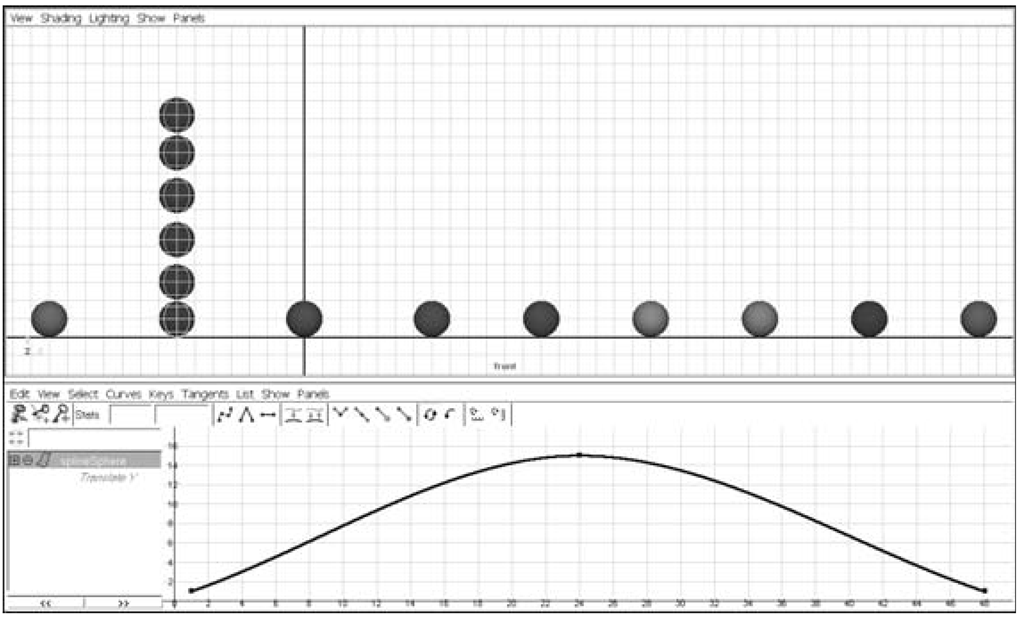
Figure 3.41: Spline tangents
5. In your Layer Editor turn on the visibility for the sphereSplineLayer. A new sphere appears. Play the animation and notice the difference between the sphereLinear and the sphereSpline. Keep in mind that both of these spheres have identical keyframes set for their translateY channels — they start and stop at the exact same time.
6. Select the sphereSpline object and take a look at its function curve in the Graph Editor (see Figure 3.41). This is an example of spline tan-gency. If you do a reverse plot of the value-over-time you’ll see that the in-between values near frame 24 change very little. This corresponds to the sphere’s slowness at the top of its height. A 2D animator would achieve this with tightly spaced drawings near the keys.
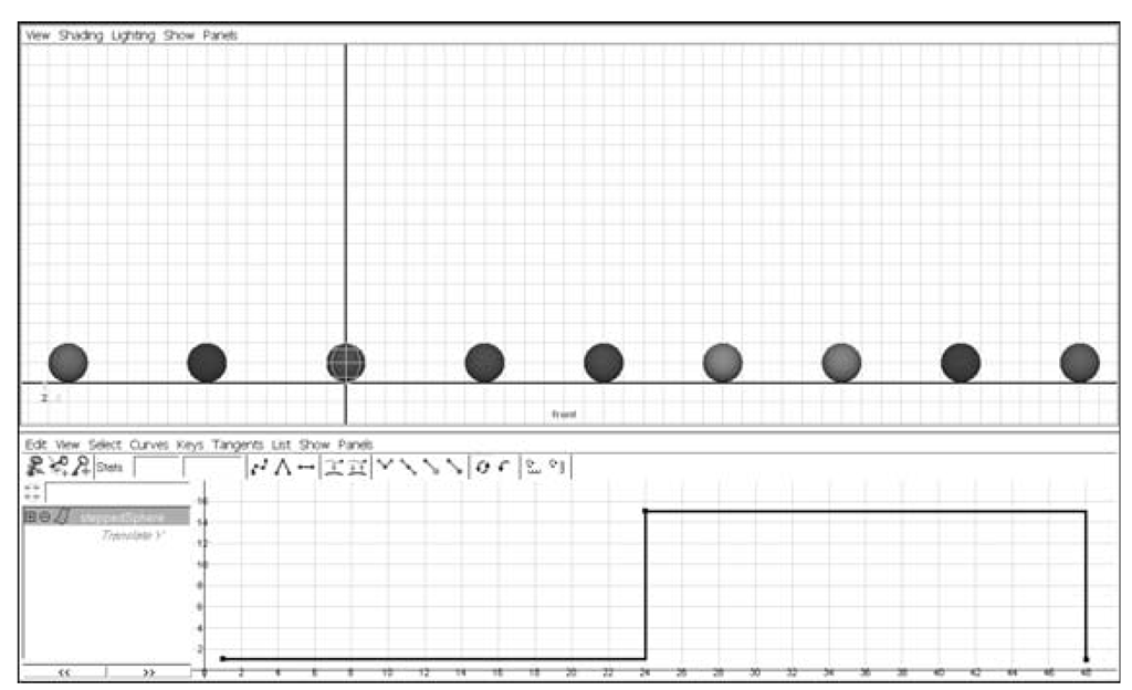
Figure 3.42: Stepped tangents
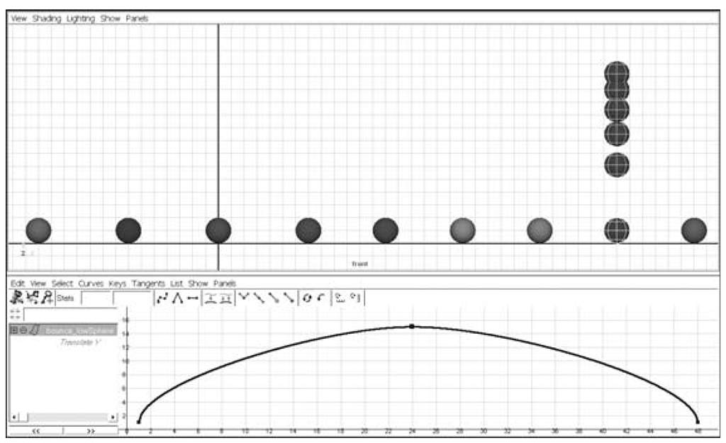
If you take a good look at the sphereSpline object’s motion it seems to ease its way into and out of the middle keyframe. This ease-in and -out (also called slow-in and -out) is the default motion a spline interpolation will give you.
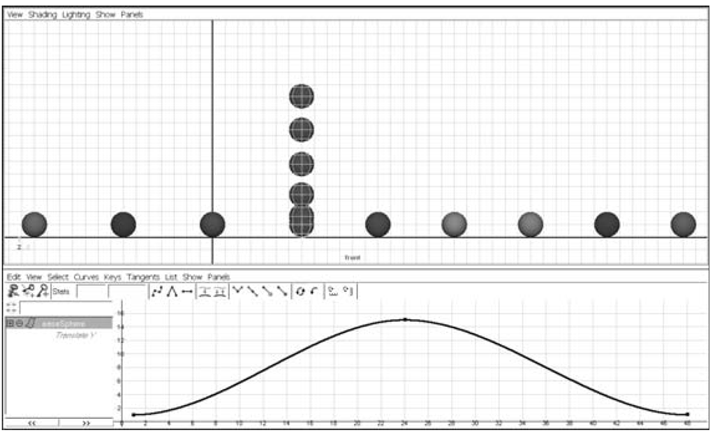
Figure 3.43: Slow-in and slow-out tangents
7. Using the Layer Editor again, make the sphereSteppedLayer visible. Play the animation and watch the third ball. This one seems to “pop” from position to position.
Take a look at the sphereStepped object’s function curve (see Figure 3.42). Rather than making any gradual value changes from frame to frame, stepped tangency holds the value at a constant right up until the moment it changes. This is useful for things such as blocking out an animation, blinking lights, and hiding things through their visibility channel.
8. Linear, spline, and stepped are the main curve tangency types. You can vary the in- and out-tan-gency for any keyframe, not just the entire curve.
Figure 3.44: Fast-in and fast-out tangents
By altering the direction and weight of a spline tangency, you can create other types of motion. In the Layer Editor, turn on the visibility of the slow_in_outLayer.
9. Select the sphereSlow object and look at its function curve (see Figure 3.43). Similar to spline tangency, this flat tan-gency makes the curve slow into and out of each keyframe. There will be gradual acceleration and gradual deceleration at all value changes.
Figure 3.45: Sticky tangents
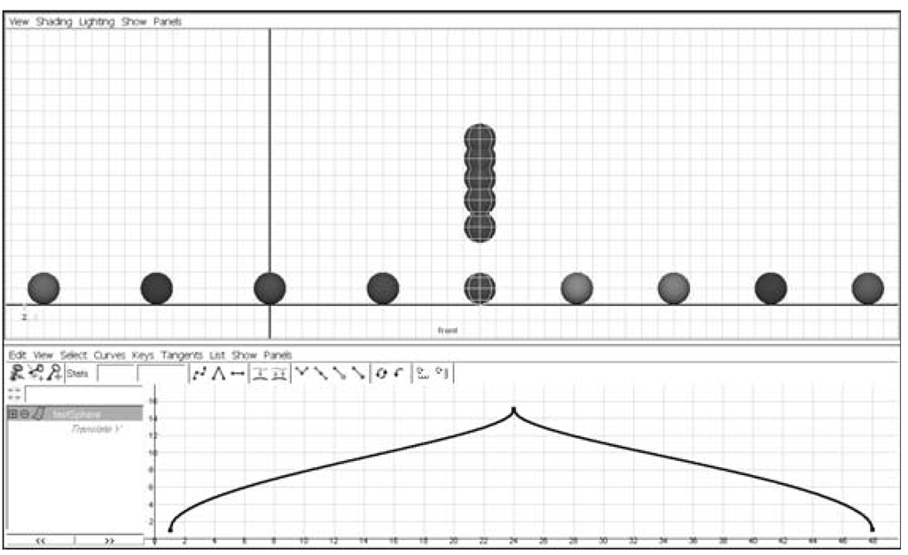
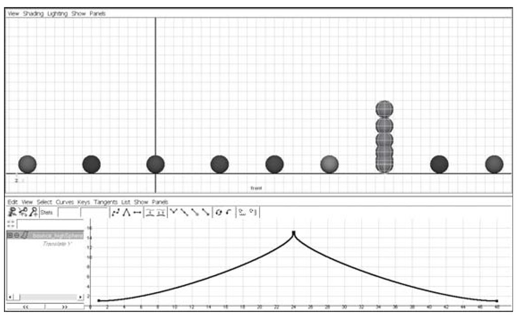
10. Turn on the visibility of the fast_in_outLayer. Select sphereFast and look at its curve (see Figure 3.44). Based on spline tangency, these in-betweens have large value changes from frame to frame. This causes rapid acceleration and rapid deceleration at the keyframes. In traditional animation this is the equivalent of drawings that are spaced far apart. Fast-in and -out tangency is achieved by breaking the tan-gency of the curve at a keyframe. We’ll look at how to do this in the next exercise.
Figure 3.46: Inverted bounce tangents
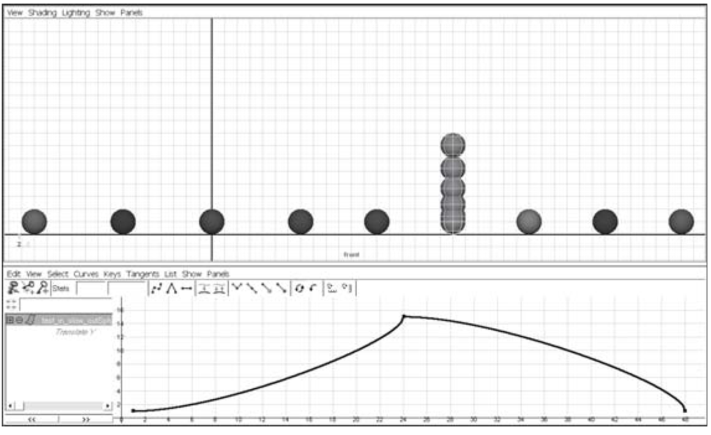
11. Turn on the visibility of the four remaining layers. These spheres all have variations on spline tangency. By breaking and varying the direction and weight of the function curves, it is possible to make the sphere rapidly accelerate, stick to the ceiling, and then gently drop (fast-in, slow-out), bounce off the ceiling (bounce-high), bounce off of the floor (bounce-low), and anticipate and overshoot its positions (see Figures 3.45 – 3.48).
Figure 3.47: Hang-time tangents
Figure 3.48: Overshooting tangents
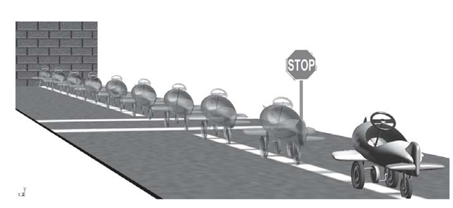
Figure 3.49: Linear plane animation
