L’Abbe plot:
A plot often used in the meta-analysis of clinical trials where the outcome is a binary response. The event risk (number of events/number of patients in a group) in the treatment groups are plotted against the risk for the controls of each trial. If the trials are fairly homogeneous the points will form a ‘cloud’ close to a line, the gradient of which will correspond to the pooled treatment effect. Large deviations or scatter would indicate possible heterogeneity.
Labour force survey:
A survey carried out in the UK on a quarterly basis since the spring of 1992. It covers 60000 households and provides labour force and other details for about 120000 people aged 16 and over. The survey covers not only unemployment, but employment, self-employment, hours of work, redundancy, education and training.
Lack of memory property:
A property possessed by a random variable Y, namely that
Variables having an exponential distribution have this property, as do those following a geometric distribution.
Lagging indicators:
Part of a collection of economic time series designed to provide information about broad swings in measures of aggregate economic activity known as business cycles. Used primarily to confirm recent turning points in such cycles. Such indicators change after the overall economy has changed and examples include labour costs, business spending and the unemployment rate.
Lagrange multipliers:
A method of evaluating maxima or minima of a function of possibly several variables, subject to one or more constraints. [Optimization, Theory and Applications, 1979, S.S. Rao, Wiley Eastern, New Delhi.]
Lagrange multiplier test:
Synonym for score test.
Lancaster, Henry Oliver (1913-2001):
Born in Kempsey, New South Wales, Lancaster intended to train as an actuary, but in 1931 enrolled as a medical student at the University of Sydney, qualifying in 1937. Encountering Yule’s Introduction to the Theory of Statistics, he became increasingly interested in statistical problems, particularly the analysis of 2 x 2 x 2 tables. After World War II this interest led him to obtain a post as Lecturer in Statistics at the Sydney School of Public Health and Tropical Medicine. In 1948 Lancaster left Australia to study at the London School of Hygiene and Tropical Medicine under Bradford Hill, returning to Sydney in 1950 to study trends in Australian mortality. Later he undertook more theoretical work that led to his 1969 topic, The Chi-squared Distribution. In 1966 he was made President of the Statistical Society of Australia. Lancaster died in Sydney on 2 December 2001.
Lancaster models:
A means of representing the joint distribution of a set of variables in terms of the marginal distributions, assuming all interactions higher than a certain order vanish. Such models provide a way to capture dependencies between variables without making the sometimes unrealisitic assumptions of total independence on the one hand, yet having a model that does not require an unrealistic number of observations to provide precise parameter estimates.
Landmark analysis:
A term applied to a form of analysis occasionally applied to data consisting of survival times in which a test is used to assess whether ‘treatment’ predicts subsequent survival time among subjects who survive to a ‘landmark’ time (for example, 6 months post-randomization) and who have, at this time, a common prophylaxis status and history of all other covariates.
Landmark registration:
A method for aligning the profiles in a set of repeated measures data, for example human growthcurves, by identifying the timing of salient features such as peaks, troughs, or inflection points. Curves are then aligned by transforming individual time so that landmark events become synchronized.
Laplace distribution:
The probability distribution, f (x), given by
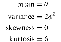
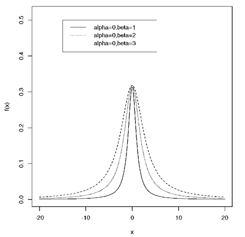
Can be derived as the distribution of the difference of two independent random variables each having an identical exponential distribution. Examples of the distribution are shown in Fig. 83. The mean, variance, skewness and kurtosis of the distribution are as follows:
Also known as the double exponential distribution.
Laplace, Pierre-Simon, Marquis de (1749-1827):
Born in Beaumont-en-Auge near to Caen where he first studied, Laplace made immense contributions to physics, particularly astronomy, and mathematics. Became a professor at the Ecole Militaire in 1771 and entered the Academie des Sciences in 1773. Most noted for his five-volume work Traite de Mecanique Celeste he also did considerable work in probability including independently discovering Bayes’ theorem, ten years after Bayes’ essay on the topic. Much of this work was published in Theorie Analytique des Probabilites. Laplace died on 5 March 1827, in Paris.
Large sample method:
Any statistical method based on an approximation to a normal distribution or other probability distribution that becomes more accurate as sample size increases. See also asymptotic distribution.
Lasagna’s law:
Once a clinical trial has started the number of suitable patients dwindles to a tenth of what was calculated before the trial began.
Fig. 83 Laplace distributions for a = 0; p = 1, 2, 3.
Lasso:
A penalized least squares regression method that does both continuous shrinkage and automatic variable selection simultaneously. It minimizes the usual sum of squared errors, with a bound on the sum of the absolute values of the coefficients. When the bound is large enough, the constraint has no effect and the solution is simply that of multiple regression. When, however, the bound is smaller, the solutions are ‘shrunken’ versions of the least squares estimates.
Last observation carried forward:
A method for replacing the observations of patients who drop out of a clinical trial carried out over a period of time. It consists of substituting for each missing value the subject’s last available assessment of the same type. Although widely applied, particularly in the pharmaceutical industry, its usefulness is very limited since it makes very unlikely assumptions about the data, for example, that the (unobserved) post drop-out response remains frozen at the last observed value. See also imputation.
Latent class analysis:
A method of assessing whether a set of observations involving categorical variables, in particular, binary variables, consists of a number of different groups or classes within which the variables are independent. Essentially a finite mixture model in which the component distributions are multivariate Bernoulli. Parameters in such models can be estimated by maximum likelihood estimation via the EM algorithm. Can be considered as either an analogue of factor analysis for categorical variables, or a model of cluster analysis for such data. See also grade of membership model.
Latent class identifiability display:
A graphical diagnostic for recognizing weakly identified models in applications of latent class analysis.
Latent moderated structural equations:
A refinement of structural equation modeling for models with multiple latent interaction effects.
Latent period:
The time interval between the initiation time of a disease process and the time of the first occurrence of a specifically defined manifestation of the disease. An example is the period between exposure to a tumorigenic dose of radioactivity and the appearance of tumours.
Latent root distributions:
Probability distributions for the latent roots of a square matrix whose elements are random variables having a joint distribution. Those of primary importance arise in multivariate analyses based on the assumption of multivariate normal distributions. See also Bartlett’s test for eigenvalues.
Latent roots:
Synonym for eigenvalues.
Latent variable:
A variable that cannot be measured directly, but is assumed to be related to a number of observable or manifest variables. Examples include racial prejudice and social class. See also indicator variable.
Latent vectors:
Synonym for eigenvectors.
Latin hypercube sampling (LHS):
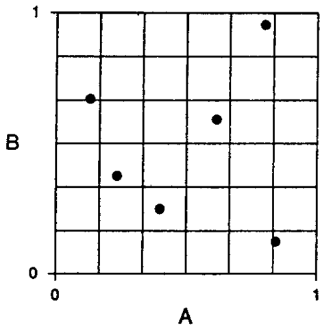
A stratified random sampling technique in which a sample of size N from multiple (continuous) variables is drawn such that for each individual variable the sample is (marginally) maximally stratified, where a sample is maximally stratified when the number of strata equals the sample size N and when the probability of falling in each of the strata equals N_1. An example is shown in Fig. 84, involving two independent uniform [0,1] variables, the number of categories per variable equals the sample size (6), each row or each column contains one element and the width of rows and columns is 1/6.
Latin square:
An experimental design aimed at removing from the experimental error the variation from two extraneous sources so that a more sensitive test of the treatment effect can be achieved. The rows and columns of the square represent the levels of the two extraneous factors. The treatments are represented by Roman letters arranged so that no letter appears more than once in each row and column. The following is an example of a 4 x 4 Latin square
| A | B | C | D |
| B | C | D | A |
| C | D | A | B |
| D | A | B | C |
Fig. 84 Latin hypercube sampling.
Lattice designs:
A class of incomplete block designs introduced to increase the precision of treatment comparisons in agricultural crop trials.
Lattice distribution:
A class of probability distributions to which most distributions for discrete random variables used in statistics belong. In such distributions the intervals between values of any one random variable for which there are non-zero probabilities are all integral multiples of one quantity. Points with these coordinates thus form a lattice. By an approximate linear transformation it can be arranged that all variables take values which are integers.
Lattice square:
An incomplete block design for v = (s — 1)s treatments in b = rs blocks, each containing s — 1 units. In addition the blocks can be arranged into r complete replications.
Law of large numbers:
A ‘law’ that attempts to formalize the intuitive notion of probability which assumes that if in n identical trials an event A occurs nA times, and if n is very large, then nA/n should be near the probability of A. The formalization involves translating ‘identical trials’ as Bernoulli trials with probability p of a success. The law then states that as n increases, the probability that the average number of successes deviates from p by more then any preassigned value e where e > 0 is arbitrarily small but fixed, tends to zero.
Law of likelihood:
Within the framework of a statistical model, a particular set of data supports one statistical hypothesis better than another if the likelihood of the first hypothesis, on the data, exceeds the likelihood of the second hypothesis.
Law of primacy:
A ‘law’ relevant to work in market research which says that an individual for whom, at the moment of choice, n brands are tied for first place in brand strength chooses each of these n brands with probability 1/n.
Law of truly large numbers:
The law that says that, with a large enough sample, any outrageous thing is likely to happen. See also coincidences.
LD50:
Abbreviation for lethal dose 50.
LDU test:
A test for the rank of a matrix A using an estimate of A based on a sample of observations.
Lead time:
An indicator of the effectiveness of a screening test for chronic diseases given by the length of time the diagnosis is advanced by screening. [International Journal of Epidemiology, 1982, 11, 261-7.]
Lead time bias:
A term used particularly with respect to cancer studies for the bias that arises when the time from early detection to the time when the cancer would have been symptomatic is added to the survival time of each case.
Leaps-and-bounds algorithm:
An algorithm used to find the optimal solution in problems that may have a very large number of possible solutions. Begins by splitting the possible solutions into a number of exclusive subsets and limits the number of subsets that need to be examined in searching for the optimal solution by a number of different strategies. Often used in all subsets regression to restrict the number of models that have to be examined. [ARA Chapter 7.]
Least absolute deviation regression:
An alternative to least squares estimation for determining the parameters in multiple regression. The criterion minimized to find the estimators of the regression coefficients is S, given by;
where yi and Xj, j = 1,…, q are the response variable and explanatory variable values for individual i. The estimators, b0, b1,…, bq of the regression coefficients, P0, …, Pq are such that the median(bj) = (median unbiased) and are maximum likelihood estimators when the errors have a Laplace distribution. Thi s type of regression has greater power than that based on least squares for asymmetric error distributions and heavy tailed, symmetric error distributions; it also has greater resistance to the influence of a few outlying values of the dependent variable.
Least significant difference test:
An approach to comparing a set of means that controls the familywise error rate at some particular level, say a. The hypothesis of the equality of the means is tested first by an a-level F-test. If this test is not significant, then the procedure terminates without making detailed inferences on pairwise differences; otherwise each pairwise difference is tested by an a-level, Student’s t-test.
Least squares cross-validation:
A method of cross validation in which models are assessed by calculating the sum of squares of differences between the observed values of a subset of the data and the relevant predicted values calculated from fitting a model to the remainder of the data.
Least squares estimation:
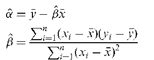
A method used for estimating parameters, particularly in regression analysis, by minimizing the difference between the observed response and the value predicted by the model. For example, if the expected value of a response variable y is of the form
where x is an explanatory variable, then least squares estimators of the parameters a and p may be obtained from n pairs of sample values (x1, y1), (x2, y2),…, (xn, yn) by minimizing S given by
to give
Often referred to as ordinary least squares to differentiate this simple version of the technique from more involved versions such as, weighted least squares and iteratively reweighted least squares. [ARA Chapter 1.]
LeCam, Lucien (1924-2000):
Born in Felletin, France, LeCam studied at the University of Paris and received a Licence en Sciences (university diploma) in 1945. His career began with work on power and hydraulic systems at the Electricite de France, but in 1950 he went to Berkeley at the invitation of Jerzy Neyman. LeCam received a Ph.D. from the university in 1952. He was made assistant Professor of Mathematics in 1953 and in 1955 joined the new Department of Statistics at Berkeley. He was departmental chairman from 1961 to 1965. LeCam was a brilliant mathematician and made important contributions to the asymptotic theory of statistics, much of the work being published in his topic Asymptotic Methods in Statistical Decision Theory, published in 1986.
Length-biased data:
Data that arise when the probability that an item is sampled is proportional to its length. A prime example of this situation occurs in renewal theory where inter-event time data are of this type if they are obtained by sampling lifetimes in progress at a randomly chosen point in time.
Length-biased sampling:
The bias that arises in a sampling scheme based on patient visits, when some individuals are more likely to be selected than others simply because they make more frequent visits. In a screening study for cancer, for example, the sample of cases detected is likely to contain an excess of slow-growing cancers compared to the sample diagnosed positive because of their symptoms.
Lepage test:
A distribution free test for either location or dispersion. The test statistic is related to that used in the Mann-Whitney test and the Ansari-Bradley test.
Leslie matrix model:
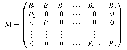
A model often applied in demographic and animal population studies in which the vector of the number of individuals of each age at time t, Nt, is related to the initial number of individuals of each age, N0, by the equation
where M is what is known as the population projection matrix given by
where Bx equals the number of females born to females of age x in one unit of time that survive to the next unit of time, Px equals the proportion of females of age x at time t that survive to time t + 1 and v is the greatest age attained. See also population growth model.
Lethal dose 50:
The administered dose of a compound that causes death to 50% of the animals during a specified period, in an experiment involving toxic material.
Levene test:
A test used for detecting heterogeneity of variance, which consists of an analysis of variance applied to residuals calculated as the differences between observations and group means.
Leverage points:
A term used in regression analysis for those observations that have an extreme value on one or more explanatory variables. The effect of such points is to force the fitted model close to the observed value of the response leading to a small residual. See also hat matrix, influence statistics and Cook’s distance. [ARA Chapter 10.]
Levy concentration function:
A function Q(x; A) of a random variable X defined by the equality
Levy concentration function:
A function Q(x; A) of a random variable X defined by the equality
for every X > 0; Q(X; A) is a non-decreasing function of X satisfying the inequalities 0 < Q(X; X) < 1 for every X > 0. A measure of the variability of the random variable that is used to investigate convergence problems for sums of independent random variables.
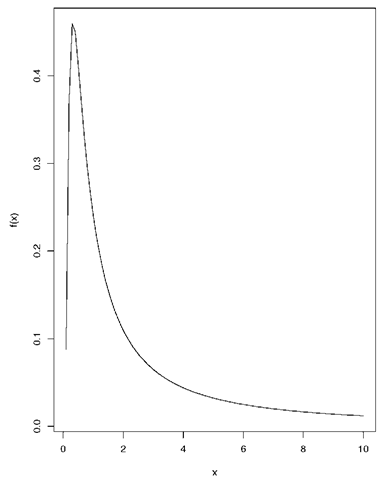
Levy distribution:
A probability distribution, f (x), given by
None of the moments of the distribution exist. An example of such a distribution is given in Fig. 85.
Levy, Paul-Pierre (1886-1971):
Born in Paris, Levy was educated at the Ecole Polytechnique between 1904 and 1906. His main work was in the calculus of probability where he introduced the characteristic function, and in Markov chains, martingales and game theory. Levy died on 15 December 1971 in Paris.
Lexian distributions:
Finite mixture distributions having component binomial distributions with common n.
Fig. 85 An example of a Levy distribution.
Lexicostatistics:
A term sometimes used for investigations of the evolution times of languages, involving counting the number of cognate words shared by each pair of present-day languages and using these data to reconstruct the ancestry of the family.
Lexis diagram:
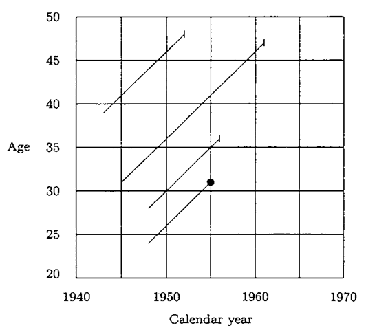
A diagram for displaying the simultaneous effects of two time scales (usually age and calendar time) on a rate. For example, mortality rates from cancer of the cervix depend upon age, as a result of the age-dependence of the incidence, and upon calendar time as a result of changes in treatment, population screening and so on. The main feature of such a diagram is a series of rectangular regions corresponding to a combination of two time bands, one from each scale. Rates for these combinations of bands can be estimated by allocating failures to the rectangles in which they occur and dividing the total observation time for each subject between rectangles according to how long the subjects spend in each. An example of such a diagram is given in Fig. 86. [Statistics in Medicine, 1987, 6, 449-68.]
Lexis, Wilhelm (1837-1914):
Lexis’s early studies were in science and mathematics. He graduated from the University of Bonn in 1859 with a thesis on analytic mechanics and a degree in mathematics. In 1861 he went to Paris to study social science and his most important statistical work consisted of several articles published between 1876 and 1880 on population and vital statistics.
Fig. 86 A Lexis diagram showing age and calendar period.
Liddell, Francis Douglas Kelly (1924-2003):
Liddell was educated at Manchester Grammar School from where he won a scholarship to Trinity College, Cambridge, to study mathematics. He graduated in 1945 and was drafted into the Admiralty to work on the design and testing of naval mines. In 1947 he joined the National Coal Board where in his 21 years he progressed from Scientific Officer to Head of the Mathematical Statistics Branch. In 1969 Liddell moved to the Department of Epidemiology at McGill University, where he remained until his retirement in 1992. Liddell contributed to the statistical aspects of investigations of occupational health, particularly exposure to coal, silica and asbestos. He died in Wimbledon, London, on 5 June 2003.
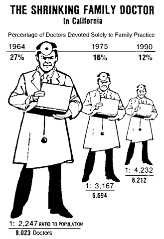
Lie factor:
A quantity suggested by Tufte forjudging the honesty of a graphical presentation of data. Calculated as apparent size of effect shown in graph actual size of effect in data Values close to one are desirable but it is not uncommon to find values close to zero and greater than five. The example shown in Fig. 87 has a lie factor of about 2.8.
Life expectancy:
The expected number of years remaining to be lived by persons of a particular age. For example, according to the US life table for 1979-1981 the life expectancy at birth is 73.88 years and that at age 40 is 36.79 years. The life expectancy of a population is a general indication of the capability of prolonging life. It is used to identify trends and to compare longevity. [Population and Development Review, 1994, 20, 57-80.1
Fig. 87 A diagram with a lie factor of 2.8.
Life table:
A procedure used to compute chances of survival and death and remaining years of life, for specific years of age. An example of part of such a table is as follows:
Life table for white females, United States, 1949-1951
| 1 | 2 | 3 | 4 | 5 | 6 | 7 |
| 0 | 23.55 | 100000 | 2355 | 97965 | 7203179 | 72.03 |
| 1 | 1.89 | 97465 | 185 | 97552 | 7105214 | 72.77 |
| 2 | 1.12 | 97460 | 109 | 97406 | 7007662 | 71.90 |
| 3 | 0.87 | 97351 | 85 | 97308 | 6910256 | 70.98 |
| 4 | 0.69 | 92266 | . 67 | 97233 | 6812948 | 70.04 |
| 100 | 388.39 | 294 | 114 | 237 | 566 | 1.92 |
| 1= | Year of age | |||||
| 2= | Death rate per | 1000 |
3 = Number surviving of 100 000 born alive
4 = Number dying of 100 000 born alive
5 = Number of years lived by cohort
6 = Total number of years lived by cohort until all have died
7 = Average future years of life
Life table analysis:
A procedure often applied in prospective studies to examine the distribution of mortality and/or morbidity in one or more diseases in a cohort study of patients over a fixed period of time. For each specific increment in the follow-up period, the number entering the period, the number leaving during the period, and the number either dying from the disease (mortality) or developing the disease (morbidity), are all calculated. It is assumed that an individual not completing the follow-up period is exposed for half this period, thus enabling the data for those 'leaving' and those 'staying' to be combined into an appropriate denominator for the estimation of the percentage dying from or developing the disease. The advantage of this approach is that all patients, not only those who have been involved for an extended period, can be be included in the estimation process.
Likelihood:
The probability of a set of observations given the value of some parameter or set of parameters. For example, the likelihood of a random sample of n observations, x1, x2,..., xn with probability distribution, f (x, 6) is given by
This function is the basis of maximum likelihood estimation. In many applications the likelihood involves several parameters, only a few of which are of interest to the investigator. The remaining nuisance parameters are necessary in order that the model make sense physically, but their values are largely irrelevant to the investigation and the conclusions to be drawn. Since there are difficulties in dealing with likelihoods that depend on a large number of incidental parameters (for example, maximizing the likelihood will be more difficult) some form of modified likelihood is sought which contains as few of the uninteresting parameters as possible. A number of possibilities are available. For example, the marginal likelihood (often also called the restricted likelihood), eliminates the nuisance parameters by transforming the original variables in some way, or by working with some form of marginal variable. The profile likelihood with respect to the parameters of interest, is the original likelihood, partially maximized with respect to the nuisance parameters. See also quasi-likelihood, conditional likelihood, law of likelihood and likelihood ratio. [KA2 Chapter 17.]
Likelihood distance test: A
procedure for the detection of outliers that uses the difference between the log-likelihood of the complete data set and the log-likelihood when a particular observation is removed. If the difference is large then the observation involved is considered an outlier.
Likelihood principle:
Within the framework of a statistical model, all the information which the data provide concerning the relative merits of two hypotheses is contained in the likelihood ratio of these hypotheses on the data.
Likelihood ratio:
The ratio of the likelihoods of the data under two hypotheses, H0 and H1. Can be used to assess H0 against H1 since under H0, the statistic, X, given by
has approximately a chi-squared distribution with degrees of freedom equal to the difference in the number of parameters in the two hypotheses. See also G2, deviance, goodness-of-fit and Bartlett’s adjustment factor.
Likert, Rensis (1903-1981):
Likert was born in Cheyenne, Wyoming and studied civil engineering and sociology at the University of Michigan. In 1932 he obtained a Ph.D. at Columbia University’s Department of Psychology. His doctoral research dealt with the measurement of attitudes. Likert’s work made a tremendous impact on social statistics and he received many honours, including being made President of the American Statistical Association in 1959.
Likert scales:
Scales often used in studies of attitudes in which the raw scores are based on graded alternative responses to each of a series of questions. For example, the subject may be asked to indicate his/her degree of agreement with each of a series of statements relevant to the attitude. A number is attached to each possible response, e.g. 1:strongly approve; 2:approve; 3:undecided; 4:disapprove; 5:strongly disapprove; and the sum of these used as the composite score. A commonly used Likert-type scale in medicine is the Apgar score used to appraise the status of newborn infants. This is the sum of the points (0,1 or 2) allotted for each of five items:
• heart rate (over 100 beats per minute 2 points, slower 1 point, no beat 0);
• respiratory effort;
• muscle tone;
• response to simulation by a catheter in the nostril;
• skin colour.
Lim-Wolfe test:
A rank based multiple test procedure for identifying the dose levels that are more effective than the zero-dose control in randomized block designs, when it can be assumed that the efficacy of the increasing dose levels in monotonically increasing up to a point, followed by a monotonic decrease.
Lindley’s paradox:
A name used for situations where using Bayesian inference suggests very large odds in favour of some null hypothesis when a standard sampling-theory test of significance indicates very strong evidence against it.
Linear birth process:
Synonym for Yule-Furry process.
Linear-by-linear association test:
A test for detecting specific types of departure from independence in a contingency table in which both the row and column categories have a natural order. See also Jonckheere-Terpstra test.
Linear-circular correlation:
A measure of correlation between an interval scaled random variable X and a circular random variable, ©, lying in the interval (0, 2n). For example, X may refer to temperature and © to wind direction. The measure is given by
where p12 = corr(X, cos ©), p13 = corr(X, sin ©) and p23 = corr(cos ©, sin ©). The sample quantity RXe is obtained by replacing the py by the sample coefficients r y.
Linear estimator:
An estimator which is a linear function of the observations, or of sample statistics calculated from the observations.
Linear filters:
Suppose a series {xt} is passed into a ‘black box’ which produces {yt} as output.
If the following two restrictions are introduced:
(1) The relationship is linear; (2) The relationship is invariant over time, then for any t, yt is a weighted linear combination
of past and future values of the input
It is this relationship which is known as a linear filter. If the input series has power spectrum hx(w) and the output a corresponding spectrum hy(!), they are related by
If we write hy(w) = \T(w)\2hx(w) where r(&>) = J2j=-1 aje j!, then r(&>) is called the transfer function while \ r(&>) is called the amplitude gain. The squared value is known as the gain or the power transfer function of the filter. [TMS Chapter 2.]
Linear function:
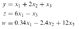
A function of a set of variables, parameters, etc., that does not contain powers or cross-products of the quantities. For example, the following are all such functions of three variables, x1, x2 and x3,
Linearizing:
The conversion of a non-linear model into one that is linear, for the purpose of simplifying the estimation of parameters. A common example of the use of the procedure is in association with the Michaelis-Menten equation
where B and F are the concentrations of bound and free ligand at equilibrium, and the two parameters, Bmax and KD are known as capacity and affinity. This equation can be reduced to a linear form in a number of ways, for example
is linear in terms of the variables 1/B and 1/F. The resulting linear equation is known as the Lineweaver-Burk equation.
Linear logistic regression:
Synonym for logistic regression.
Linearly separable:
A term applied to two groups of observations when there is a linear function of a set of variables x’ = [x1, x2,..., xq], say, x’a + b which is positive for one group and negative for the other. See also discriminant function analysis and Fisher’s linear discriminant function. [Investigative Ophthalmology and Visual Science, 1997, 38, 4159.]
Linear model:
A model in which the expected value of a random variable is expressed as a linear function of the parameters in the model. Examples of linear models are
where x and y represent variable values and a, fi and y parameters. Note that the linearity applies to the parameters not to the variables. See also linear regression and generalized linear models. [ARA Chapter 6.]
Linear regression:
A term usually reserved for the simple linear model involving a response, y, that is a continuous variable and a single explanatory variable, x, related by the equation
Linear transformation:
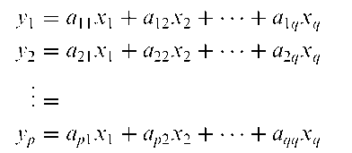
A transformation of q variables x1, x2,…, xq given by the q equations
Such a transformation is the basis of principal components analysis.
Linear trend:
A relationship between two variables in which the values of one change at a constant rate as the other increases.
Line-intercept sampling:
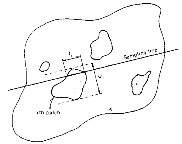
A method of unequal probability sampling for selecting sampling units in a geographical area. A sample of lines is drawn in a study region and, whenever a sampling unit of interest is intersected by one or more lines, the characteristic of the unit under investigation is recorded. The procedure is illustrated in Fig. 88. As an example, consider an ecological habitat study in which the aim is to estimate the total quantity of berries of a certain plant species in a specified region. A random sample of lines each of the same length is selected and drawn on a map of the region. Field workers walk each of the lines and whenever the line intersects a bush of the correct species, the number of berries on the bush are recorded. [Sampling Biological Populations, 1979, edited by R.M. Cormack, G.P. Patil and D.S. Robson, International Co-operative Publishing House, Fairland.]
Fig. 88 An illustration of line-intercept sampling.
Linkage analysis:
The analysis of pedigree data concerning at least two loci, with the aim of determining the relative positions of the loci on the same or different chromosome. Based on the non-independent segregation of alleles on the same chromosome.
Linked micromap plot:
A plot that provides a graphical overview and details for spatially indexed statistical summaries. The plot shows spatial patterns and statistical patterns while linking regional names to their locations on a map and to estimates represented by statistical panels. Such plots allow the display of confidence intervals for estimates and inclusion of more than one variable.
LISREL:
A computer program for fitting structural equation models involving latent variables.
Literature controls:
Patients with the disease of interest who have received, in the past, one of two treatments under investigation, and for whom results have been published in the literature, now used as a control group for patients currently receiving the alternative treatment. Such a control group clearly requires careful checking for comparability. See also historical controls.
Lobachevsky distribution:
The probability distribution of the sum (X) of n independent random variables, each having a uniform distribution over the interval [— 1,2], and given by
where [x + n/2] denotes the integer part of x + n/2.
Local dependence fuction:
An approach to measuring the dependence of two variables when both the degree and direction of the dependence is different in different regions of the plane.
Locally weighted regression:
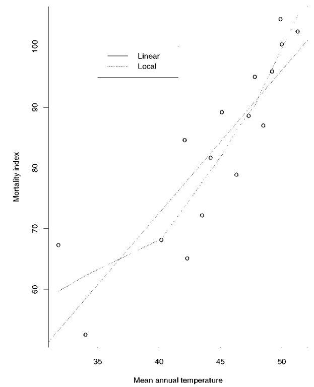
A method of regression analysis in which polynomials of degree one (linear) or two (quadratic) are used to approximate the regression function in particular ‘neighbourhoods’ of the space of the explanatory variables. Often useful for smoothing scatter diagrams to allow any structure to be seen more clearly and for identifying possible non-linear relationships between the response and explanatory variables. A robust estimation procedure (usually known as loess) is used to guard against deviant points distorting the smoothed points. Essentially the process involves an adaptation of iteratively reweighted least squares. The example shown in Fig. 89 illustrates a situation in which the locally weighted regression differs considerably from the linear regression of y on x as fitted by least squares estimation. See also kernel regression smoothing. [Journal of the American Statistical Association, 1979, 74, 829-36.]
Local odds ratio:
The odds ratio of the two-by-two contingency tables formed from adjacent rows and columns in a larger contingency table.
Fig. 89 Scatterplot of breast cancer mortality rate versus temperature of region with lines fitted by least squares calculation and by locally weighted regression.
Location:
The notion of central or ‘typical value’ in a sample distribution. See also mean, median and mode.
LOCF:
Abbreviation for last observation carried forward.
Lods:
A term often used in epidemiology for the logarithm of an odds ratio. Also used in genetics for the logarithm of a likelihood ratio.
Lod score:
The common logarithm (base 10) of the ratio of the likelihood of pedigree data evaluated at a certain value of the recombination fraction to that evaluated at a recombination fraction of a half (that is no linkage).
Logarithmic series distribution:
The probability distribution of a discrete random variable, X, given by
where y is a shape parameter lying between zero and one, and k = — 1/ log(l — y). The distribution is the limiting form of the negative binomial distribution with the zero class missing. The mean of the distribution is ky/(1 — y) and its variance is ky(1 — ky)/(1 — y)2. The distribution has been widely used by entomologists to describe species abundance. [STD Chapter 23.]
Logarithmic transformation:
The transformation of a variable, x, obtained by taking y = ln(x). Often used when the frequency distribution of the variable, x, shows a moderate to large degree of skewness in order to achieve normality.
Log-cumulative hazard plot:
A plot used in survival analysis to assess whether particular parametric models for the survival times are tenable. Values of ln(— ln S(t)) are plotted against ln t, where S(t) is the estimated survival function. For example, an approximately linear plot suggests that the survival times have a Weibull distribution and the plot can be used to provide rough estimates of its two parameters. When the slope of the line is close to one, then an exponential distribution is implied. [Modelling Survival Data in Medical Research, 2nd edition, 2003, D. Collett, Chapman and Hall/CRC Press, London.]
Log-F accelerated failure time model:
An accelerated failure time model with a generalized F-distribution for survival time.
Logistic distribution:
The limiting probability distribution as n tends to infinity, of the average of the largest to smallest sample values, of random samples of size n from an exponential distribution. The distribution is given by
The location parameter, a is the mean. The variance of the distribution is n f /3, its skewness is zero and its kurtosis, 4.2. The standard logistic distribution with a = 0, f = 1 with cumulative probability distribution function, F(x), and probability distribution, f (x), has the property
Logistic growth model:
The model appropriate for a growth curve when the rate of growth is proportional to the product of the size at the time and the amount of growth remaining. Specifically the model is defined by the equation
where a, f and y are parameters.
Logistic normal distributions:
A class of distributions that can model dependence more flexibly that the Dirichlet distribution.
Logistic regression:
A form of regression analysis used when the response variable is a binary variable. The method is based on the logistic transformation or logit of a proportion, namely
As p tends to 0, logit(p) tends to —1 and as p tends to 1, logit(p) tends to 1. The function logit(p) is a sigmoid curve that is symmetric about p = 0.5. Applying this transformation, this form of regression is written as;
wherep = Pr(dependent variable=1) and x1, x2,…, xq are the explanatory variables. Using the logistic transformation in this way overcomes problems that might arise if p was modelled directly as a linear function of the explanatory variables, in particular it avoids fitted probabilities outside the range (0,1). The parameters in the model can be estimated by maximum likelihood estimation. See also generalized linear models and mixed effects logistic regression. [SMR Chapter 12.]
Logit confidence limits:
The upper and lower ends of the confidence interval for the logarithm of the odds ratio, given by
where is the estimated odds ratio, za=2 the normal equivalent deviate corresponding to a value of a/2, (1 — a) being the chosen size of the confidence interval. The variance term may be estimated by
where a, b, c and d are the frequencies in the two-by-two contingency table from which ^ is calculated. The two limits may be exponentiated to yield a corresponding confidence interval for the odds ratio itself.
Logit rank plot:
A plot of logit{Pr(E|S)} against logit(r) where Pr(E|S) is the conditional probability of an event E given a risk score S and is an increasing function of S, and r is the proportional rank of S in a sample of population. The slope of the plot gives an overall measure of effectiveness and provides a common basis on which different risk scores can be compared.
Log-likelihood:
The logarithm of the likelihood. Generally easier to work with than the likelihood itself when using maximum likelihood estimation.
Log-linear models:
Models for count data in which the logarithm of the expected value of a count variable is modelled as a linear function of parameters; the latter represent associations between pairs of variables and higher order interactions between more than two variables. Estimated expected frequencies under particular models are found from iterative proportionalfitting. Such models are, essentially, the equivalent for frequency data, of the models for continuous data used in analysis of variance, except that interest usually now centres on parameters representing interactions rather than those for main effects. See also generalized linear model.
Lognormal distribution:
The probability distribution of a random variable, X, for which ln(X) has a normal distribution with mean and variance a2. The distribution is given by
The mean, variance, skewness and kurtosis of the distribution are
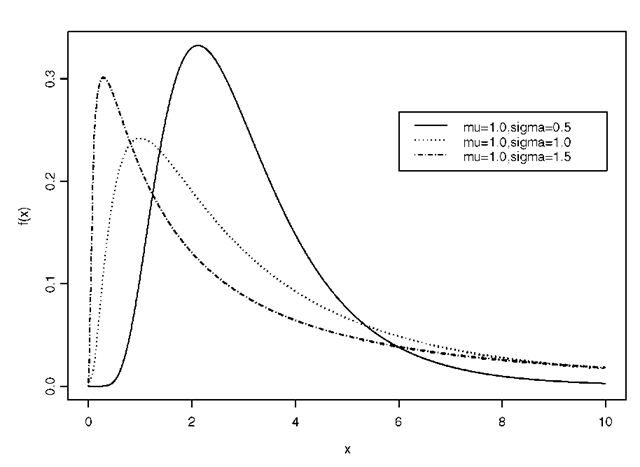
For small a the distribution is approximated by the normal distribution. Some examples of the distribution are given in Fig. 90.
Logrank test:
A test for comparing two or more sets of survival times, to assess the null hypothesis that there is no difference in the survival experience of the individuals in the different groups. For the two-group situation the test statistic is
where the weights, Wj are all unity, dy is the number of deaths in the first group at j the jth ordered death time, j = 1, 2,…, r, and e1j- is the corresponding expected number of deaths given by
where dj is the total number of deaths at time j n.j is the total number of individuals at risk at this time, and n1j- the number of individuals at risk in the first group. The expected value of U is zero and its variance is given by
Fig. 90 Lognormal distributions for ^ = 1.0; a = 0.5, 1.0, 1.5.
where
Consequently U/V V can be referred to a standard normal distribution to assess the hypothesis of interest. Other tests use the same test statistic with different values for the weights. The Tarone-Ware test, for example, uses wj = V”; and the Peto-Prentice test uses
LOGXACT:
A specialized statistical package that provides exact inference capabilities for logistic regression.
Lomb periodogram:
A generalization of the periodogram for unequally spaced time series.
Longini-Koopman model:
In epidemiology a model for primary and secondary infection, based on the characterization of the extra-binomial variation in an infection rate that might arise due to the ‘clustering’ of the infected individual within households. The assumptions underlying the model are:
• a person may become infected at most once during the course of the epidemic;
• all persons are members of a closed ‘community’. In addition each person belongs to a single ‘household’. A household may consist of one or several individuals;
• the sources of infection from the community are distributed homogeneously throughout the community. Household members mix at random within the household;
• each person can be infected either from within the household or from the community. The probability that a person is infected from the community is independent of the number of infected members in his or her household;
The probability that exactly k additional individuals will become infected for a household with s initial susceptibles and j initial infections is
where B is the probability that a susceptible individual is not infected from the community during the course of the infection, and Q is the probability that a susceptible person escapes infection from a single infected household member.
Longitudinal data:
Data arising when each of a number of subjects or patients give rise to a vector of measurements representing the same variable observed at a number of different time points. Such data combine elements of multivariate data and time series data. They differ from the former, however, in that only a single variable is involved, and from the latter in consisting of a (possibly) large number of short series, one from each subject, rather than a single long series. Such data can be collected either prospectively, following subjects forward in time, or retrospectively, by extracting measurements on each person from historical records. This type of data is also often known as repeated measures data, particularly in the social and behavioural sciences, although in these disciplines such data are more likely to arise from observing individuals repeatedly under different experimental conditions rather than from a simple time sequence. Special statistical methods are often needed for the analysis of this type of data because the set of measurements on one subject tend to be intercorrelated. This correlation must be taken into account to draw valid scientific inferences. The design of most such studies specifies that all subjects are to have the same number of repeated measurements made at equivalent time intervals. Such data is generally referred to as balanced longitudinal data. But although balanced data is generally the aim, unbalanced longitudinal data in which subjects may have different numbers of repeated measurements made at differing time intervals, do arise for a variety of reasons. Occasionally the data are unbalanced or incomplete by design; an investigator may, for example, choose in advance to take measurements every hour on one half of the subjects and every two hours on the other half. In general, however, the main reason for unbalanced data in a longitudinal study is the occurrence of missing values in the sense that intended measurements are not taken, are lost or are otherwise unavailable. See also Greenhouse and Geisser correction, Huynh-Feldt correction, compound symmetry, generalized estimating equations, Mauchly test, response feature analysis, time-by-time ANOVA and split-plot design.
Longitudinal studies:
Studies that give rise to longitudinal data. The defining characteristic of such a study is that subjects are measured repeatedly through time.
Long memory processes:
A stationary stochastic process with slowly decaying or long-range correlations. See also long-range dependence.
Long-range dependence:
Small but slowly decaying correlations in a stochastic process.
Such correlations are often not detected by standard tests, but their effect can be quite strong.
Lord, Frederic Mather (1912-2000):
Born in Hanover, New Hampshire, Lord graduated from Dartmouth College in 1936 and received a Ph.D. from Princeton in 1952. In 1944 he joined the Educational Testing Service and is recognized as the principal developer of the statistical machinery underlying modern mental testing. Lord died on 5 February 2000 in Naples, Florida.
Lord’s paradox:
A version of Simpson’s paradox.
Lorenz curve:
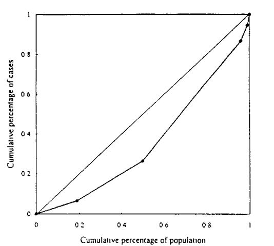
An indicator of exposure-disease association that is simply a plot of the cumulative percentage of cases against the cumulative percentage of population for increasing exposure. See Fig. 91 for an example. If the risks of disease are not monotonically increasing as the exposure becomes heavier, the data have to be rearranged from the lowest to the highest risk before the calculation of the cumulative percentages. Associated with such a curve is the Gini index defined as twice the area between the curve and the diagonal line. This index is between zero and one, with larger values indicating greater variability while smaller ones indicate greater uniformity. [KA1 Chapter 2.]
Fig. 91 Example of Lorenz curve and Gini index.
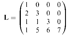
Lower triangular matrix:
A matrix in which all the elements above the main diagonal are zero. An example is the following,
LSD:
Abbreviation for least significant difference.
LST:
Abbreviation for large simple trial.
L-statistics:
Linear functions of order statistics often used in estimation problems because they are typically computationally simple.
Luganni and Rice formula:
A saddlepoint method approximation to a probability distribution from a corresponding cumulant generating function.
Lyapunov exponent: A measure of the experimental divergence of trajectories in chaotic systems [
Lynden-Bell method:
A method for estimating the hazard rate, or probability distribution of a random variable observed subject to data truncation. It is closely related to the product-limit estimator for censored data.

