Optimisation of Virtual Machine Garbage Collection Policies (Software and Computer Systems) (Analytical and Stochastic Modeling) Part 2

Heuristic for Minimal Average Response Time

In this section we discuss an application of the proposed model to define a heuristic for determining the optimum activation rate in a system with garbage collection. In practice, we aim to determine, in flight, the optimum garbage collector activation rate ai.

Assume that given a system with B available memory blocks and equipped with a garbage collector, we can measure the number of free memory blocks f, and, given this value, the average service times p,i, the average rates at which the garbage collector can free a block of memory Yi and the average rate at which the garbage collector returns control to the program /3i, where i = B — f, i.e., the number of occupied blocks. B should be chosen so that the size of each block is equal to the average memory occupation required by a customer.

Those statistics are easily measurable in many real systems, e.g., in the Sun/Oracle Java Virtual Machine using the -verbose:gc option, and can be conveniently stored in vectors of length B whose indices are the number of occupied blocks i. We should call those vectorsfor values ofand /3i, respectively. Moreover, let a be the vector of the optimal activation rates. This vector, initially, contains unknown rates

At any given time, the system could be able to measure values of only for the first k blocks of occupied memory. The remaining ratesand are then assumed as equal torespectively.

The model is then parametrised, given the measurements inas follows:

These assignments leave a set of free parameters {ai} for 1 < i < B, that have to be determined in order to fully instantiate the model. The aim of our proposed heuristic is to find an assignment for this set that minimise the average response time.

Let a’ be a vector of size B and M(a’) be the model with the parametrisation shown in Equation (9), wherei.e., where all garbage collector activation rates are parametrized using the elements of the vector. Moreover, letbe the average response time predicted using the model M (a’).

We recall that, when the condition of Equations (3) holds, we can easily compute the mean response time R = E[R] using Equations (4) and (5).

In order to make the vector a’, and thus the optimisation problem, dependent on a single variable, letbe a function that, given a positive real number, returns a vector of B real numbers such that the following proportionality condition holds:

For the sake of simplicity, in the rest of the paper we would use a function AB such thati.e., a vector where all elements are equal to a.

We have discussed the solution of the optimisation problem in the previous section in case if ai = a for all i = 1,…,N. This choice is convenient from the implementation point of view since the activation of the garbage collector is controlled by a timer which is initialised according to an exponentially distributed random delay with mean a-1, hence its activation is state-independent. Also the optimisation problem becomes easier to solve. In Section 5 we will show an example of the average response time as function of a for a special case. Nevertheless, one may decide to keep different values for ai (maybe just by speeding up the activation rate when the swap-area is approaching) and still use the fmin-con Matlab function to obtain a (sub)optimum solution. Observe that, one may wish also to consider [ i as a parameter for the optimisation, maybe introducing other constrain due to the type of applications that the server is running.

Vector a = A(ai) is then used to tune the garbage collector, i.e., to set the actual activation rates a.

It is important to recall that previsions made by our heuristic are based on incomplete data, i.e., on measurements made by the system up to k used memory blocks. The system behaviour when the memory occupancy is increased could be very different, so, in order to deal with this problem, we have to define a policy for model parametrisation updating. Whenever the system uses more than k blocks, where k is the number used for the previous parametrisation, it could determine if the estimation, for k < i < B of the values of [i, Yi and as [k, Yk and pk, respectively, are good enough, e.g., if they differ by less than a chosen percentage, or if the model has to be parametrised again in order to get better estimation for ai values, that could be then used to parametrise again the actual system, and so on, in a continuous cycle of estimation and parametrisation.

Numerical Examples

Once defined a heuristic for finding an optimal garbage collection activation rate, we should be interested in the sensitivity of this optimum in respect of other parameters. In this section we show some numerical examples obtained using our model. In order to compute these results we have used some software tools, such the library SMCSolver [1] and MATLAB.

In Figure 4 we can see how the mean response time varies in function of the garbage collection activation rate for an arrival rate A = 3. The other parameters of the model are shown in Table 1.

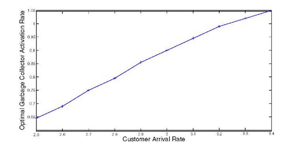
In Figure 5 we can see how the optimal garbage collector activaton rate a varies when the customer arrival rate A. As in the previous example, the other parameters of the model can be seen in Table 1.

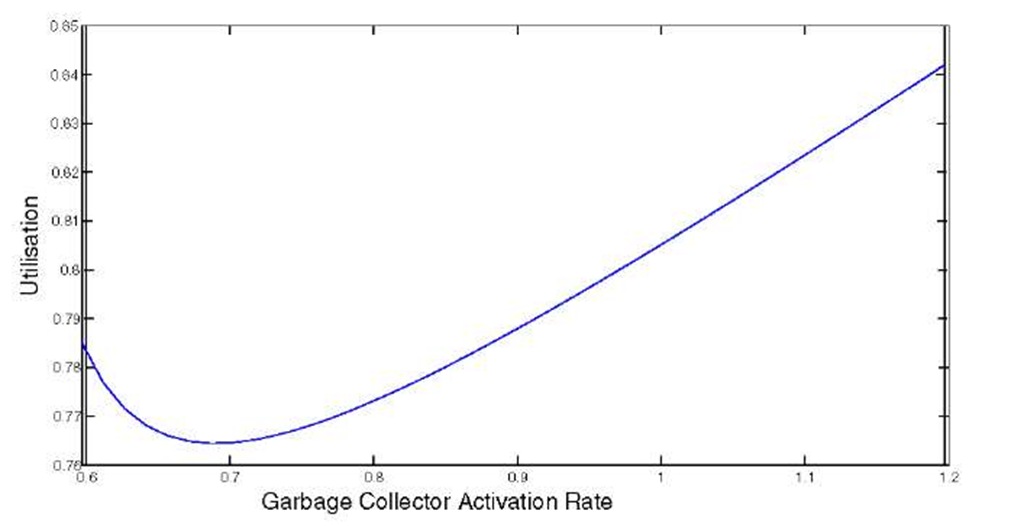
Figure 6 shows how the system utilisation p, i.e., the probability that the system is non-empty, given an arrival rate A = 3 and the other parameters as shown in Table 1, is affected by the choice of a value for the garbage collector activation rate a.

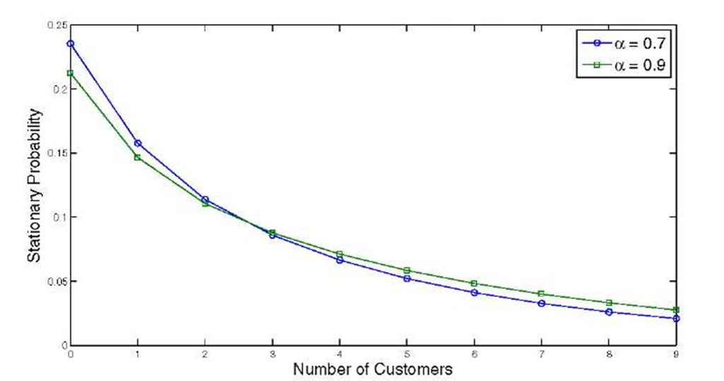
Notice that, in the previous example, the utilisation p is minimised for an a value that is different from the value that minimises the mean response time. This behaviour can be explained observing that, as shown in Figure 7, it is possible that, given two different distributionsafter a certain

Fig. 4. An example of the function R

Fig. 5. Optimal a value in function of A

Fig. 6. p value in function of a

Fig. 7. Vector n for two different a values and A = 3

Table 1. Parameter Values in Numerical Examples

Parameter Name	Value
B	50

Conclusion

In this paper we presented a queueing model of a system with garbage collection. From a theoretical point of view, the model is a Quasi-Birth&Death process, and can be studied via Matrix Geometric method. Specifically, closed expressions for the mean number of customers and the mean response time are given. The queueing model is then used to provide an estimation of the optimum garbage collection activation rate in order to minimise the mean customer response time. We showed that under a set of conditions the problem is numerically tractable with automatic tools. Finally, we proposed to use the introduced queueing model as a base for the scheduling activities of the garbage collector. To this purpose, there should be a monitor collecting system statistics on the workload of the processes. These data are used to parametrise the model and periodically determine a new optimum activation rate for the garbage collector in order to minimise the mean response time.

Future research efforts will be devoted to a stronger validation of the model with real-measurements. Moreover, we plan to compare the performance indices of traditional garbage collector activation policies with the one we proposed here.