Abstract
This paper considers a continuous-time queueing model with two types (classes) of customers each having their own dedicated server. The system adopts a "global FCFS" service discipline, i.e., all arriving customers are accommodated in one single FCFS queue, regardless of their types. As a consequence of the "global FCFS" rule, customers of one type may be blocked by customers of the other type, in that they may be unable to reach their dedicated server even at times when this server is idle, i.e., the system is basically non-workconserving. One major aim of the paper is to estimate the negative impact of this phenomenon on the (mean) system occupancy and mean system delay. For this reason, the systems with and without "global FCFS" are studied and compared. The motivation of our work are systems where this kind of blocking is encountered, such as input-queueing network switches or road splits.
Keywords: queueing; blocking; global FCFS; Markov; non-workcon-serving.
Introduction
In general, queueing phenomena occur when some kind of customers, desiring to receive some kind of service, compete for the use of a service facility (containing one or multiple servers) able to deliver the required service. Most queueing models assume that a service facility delivers exactly one type of service and that all customers requiring this type of service are accommodated in one common queue. If more than one service is needed, multiple different service facilities can be provided, i.e., one service facility for each type of service, and individual separate queues are formed in front of these service facilities. In all such models, customers are only hindered by customers that require exactly the same kind of service, i.e., that compete for the same resources.
In some applications, it may not be physically feasible or desirable to provide separate queues for each type of service that customers may require, and it may be necessary or desirable to accommodate different types of customers (i.e., customers requiring different types of service) in the same queue. In such cases, customers of one type (i.e., requiring a given type of service) may also be hindered by customers of other types. For instance, if a road or a highway is split in two or more subroads leading to different destinations, cars on that road heading for destination A may be hindered or even blocked by cars heading for destination B, even when the subroad leading to destination A is free, simply because cars that go to B are in front of them. In other words, there is a first-come-first-served (FCFS) order on the main road. This blocking also takes place in weaving sections on highways albeit to a lesser extent [1,2]. We refer to [3,4] for a general overview and validation of the modelling of traffic flows with queueing models. Similarly, in switching nodes of telecommunication networks, information packets with a given destination of node A may have to wait for the transmission of packets destined to node B that arrived earlier, even when the link to node A is free, if the arriving packets are accommodated in so-called input queues according to the source from which they originate (the well-known HOL-blocking effect, see [5,6,7,8,9]).
In order to gain insight in the impact of this kind of phenomenon on the performance of the involved systems, we analyse and compare in this paper two systems. The first system is a system where different types of customers are accommodated in the same queue and global FCFS is assumed. The second system is a system where different types of customers are still accommodated in the same queue, but without global FCFS.
Mathematical Model
We consider a continuous-time queueing model with infinite waiting room. There are two servers which both have exponential service times with mean service rate /. Each of the two servers is dedicated to a given class of customers. In this case, server A always serves customers of one type (say type 1) and server B always serves customers of a second type (type 2).
The customers enter the system according to a Poisson arrival process with mean arrival rate A. The types of consecutive customers are independent, i.e., every time a customer arrives, the customer is of type 1 with probability a and of type 2 with probability (1 — a).
In the first (and most important) model, we assume that customers all queue together and are served in the order of arrival, regardless of the class they belong to. In our paper, we will call this service discipline "global FCFS".
It can be seen that the two-server system described above is non-work conserving, for two different (orthogonal) reasons. First, the fact that the two servers A and B are dedicated to only one type of customers each, may result in situations where only one of the servers is active even though the system contains more than one customer (of the same type, in such a case). This implies that we cannot expect the system to perform as well as a regular two-server queue with two equivalent servers, i.e., servers able to serve all customers. In this paper, we consider this form of inefficiency as an intrinsic feature of our system, simply caused by the fact that the customers as well as the servers are non-identical.
The second reason why the system is non-work conserving lies in the use of the global FCFS service discipline. This rule may result in situations where only one server is active although the system contains customers of both classes. Such situations occur whenever the two customers at the front of the queue are of the same type: only one of them can then be served (by its own dedicated server) and the other "blocks" the access to the second server for customers of the opposite type further in the queue. This second form of inefficiency is not an intrinsic feature of two-class systems with dedicated servers, but rather it is due to the accidental order in which customers of both types happen to arrive (and receive service) in the system. It is this second mechanism that we want to emphasize in the paper. Therefore, we also study a system without this second mechanism in order to quantify the impact of the global FCFS rule.
The rest of this paper can be split up into three parts. In section 3, we will first discuss the system with global FCFS with a focus on the number of customers in the system and the stability of the system. This system is modelled by a continuous-time Markov chain and is solved using generating functions. Next in section 4, the system without the restriction of global FCFS will be discussed, again with a focus on the number of customers and stability of the system. Section 5 is devoted to the comparison between both systems. Some conclusions and directions for future work are given in section 6.
System with a Global FCFS Service Discipline
System State Diagram and Balance Equations
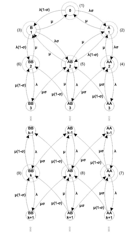
The system can be described by a continuous-time Markov chain (see Fig. 1). The states of the Markov chain contain the number of customers in the system and the types of the two customers at the front of the system. For example, the state AB(k), means that one of the customers is of type 1 (is a customer for server A) and the other customer is of type 2 (is a customer for server B), and there are a total of k customers in the system. Because, at each time, only the first two customers can be served (if they are of different types) we are only interested in the type of the customer when the customer becomes the second customer at the front of the system. This type is independent of the type of previous customers, by assumption, so the customer is of type 1 with probability a and of type 2 with probability (1 — a).
The balance equations of the state diagram of the system in Fig. 1, are
Fig. 1. State Diagram of the system with global FCFS
where
Analysis of the System
Stability Condition. Intuitively, stability means that the expected direction (drift) of the process for states in the repeating portion of the chain is towards lower valued states (lower number of customers in the system). If the chain tends to move towards higher valued states (higher number of customers in the system), then the chain is unstable. To calculate the average drift the probabilities are needed that the process is in an interlevel state j (here AA, AB or BB) of the repeating portion of the process for a level k far from the boundary, i.e., for k >> 0 (here called qj). Intuitively speaking since these levels are far from the boundary, the values qj are independent of the level k. To determine these values a derived Markov chain is considered which identifies transitions only in terms of their interlevels. Specifically, if the original process has a transition from state (k,j) tot state (k — i, l) (in this case i = —1 or 1), then in the derived process it is only considered that a transition occurs from interlevel state j to interlevel state l. [10,11]
Translated to the system in this paper, it is easily seen in Fig. 1 that the drift towards higher values and the drift towards lower values are respectively
The following equations are found by making equations (7) to (9) independent of the level k by substituting pAA(k) by qAA, PAB (k) by qAB and so forth,
This equation system lets us calculate all the probabilities (qj) to be in an interlevel state j of the repeating portion of the chain. Inserting these qj in (10) and (11) give us the stability condition,
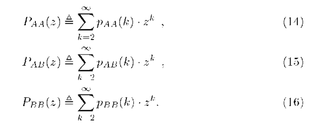
Distribution and Moments of System Occupancy. To tackle this problem, generating functions are used. We first introduce the three following partial probability generating functions (pgf’s)
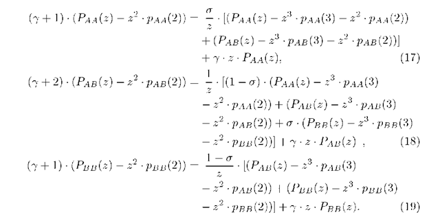
Equations (7) to (9) are multiplied by zk and summed over all k 3. We find
The common probability generating function of the (total) number of customers in the system is given by
If we solve equations (1) to (6) and (17) to (19) and insert the solutions in (20) this equation translates into a linear equation that only contains known quantities, except for two unknown probabilities in the numerator. These can be determined, in general, by invoking the well-known property that pgf’s such as P(z) are bounded inside the closed unit disk {z : \z\ < 1} of the complex z-plane, at least when the stability condition (13) of the queueing system is met (only in such a case our analysis was justified and P(z) can be viewed as a legitimate pgf).
In our case, the denominator of P(z) is of degree 5. The Abel-Ruffini theorem tells us that for a function of degree 5 or higher, it is not possible to find the zeroes explicitly.But in this case, we already know one of the five zeroes (z = 1) of the denominator so we only have to find the zeroes of a function of fourth degree which is possible by means of the method of Ferrari [15]. The denominator of P(z) is given by
and has four zeroes (besides z = 1) of the form
where the signs ±s or ±t can be plus or minus (so four options for four zeroes). We can prove that the only zero of these four zeroes, named z0 in the rest of the paper, that is inside the closed unit disk when the stability condition is met, is the zero where ±s = — and ±t = +.
It is clear that this first zero (zo) should also be a zero of the numerator of (20), as P(z) must remain bounded in this point (inside the closed unit disk). The requirement that the numerator should vanish yields a linear equation for the two unknowns. For the zero z = 1, this condition is fulfilled regardless of the values of the unknowns, since the numerator of (20) contains a factor z — 1. A second linear equation can however be obtained by invoking the normalizing condition of the pgf P(z), i.e., the condition P(1) = 1. In general, the two unknown probabilities can be found as the solutions of the two established linear equations. Substitution of the obtained values in (20) then leads to a fully determined and explicit expression for the steady-state pgf P(z) of the system occupancy.
From this result, various performance measures of practical importance can then be derived. For instance, the mean system occupancy can be found as N = P’(1). The mean system delay can then be calculated using Little’s Law [16].
System without Global FCFS
Network Model
When the global FCFS restriction is dropped and replaced by the service discipline FCFS for each of the types separately (i.e., a customer can be served if no customers of his own type are in front of him), our system is equivalent to a network of two parallel, separate queues (see Fig. 2) where each customer upon arrival goes immediately to the queue (waiting room) for its own server. The analysis of this model turns out to be much easier.
Analysis of the System
The random split property of the Poisson process (stating that if a Poisson process with intensity A is randomly split into two subprocesses with probabilities a and (1 — a), then the resulting processes are independent Poisson processes with intensities a • A and (1 — a) • A) makes the network meet the requirements of a Jackson network [17].
Fig. 2. Network model of the system without global FCFS
The fact that the system is a Jackson network, greatly simplifies the analysis of this network. The following traffic equations of the system in this paper are very simple
and the mean service rates of the servers are given by
The Jackson’s theorem states (for our case) that if (and only if) the unique solution of the traffic equations (Aj) satisfies
then the network possesses stochastic equilibrium and a steady-state distribution of the state of the Jackson network is given by a product form
where the left side of the equation is the joint distribution to have ki customers in node (queue) 1 and k2 in node (queue) 2. The right side of the equation is the product of the marginal distributions to have ki customers in node (queue) i of the network of queues.
So the network can be split in two simple M/M/ 1-queues and the marginal distributions of those queues can be multiplied to get the joint distribution. The solution of a simple M/M/ 1-queue is well-known from many topics about queueing theory e.g. [18]. The solutions of the two queues (one for server A and one for server B) are given in (27) and (28). The notation y is again introduced and is defined as in section 3.
The stability condition for the system exists out of merging the stability conditions of the two queues separately ((30) and (31)). Those stability conditions are also the conditions that must be met to be able to use Jackson’s Theorem.
After merging, this gives the stability condition for the system
The mean system occupancy N and, with use of Little’s Law, the mean delay T of a customer are respectively given by


