Neighborhood Processing (Introduction to Video and Image Processing) Part 3

Gradients

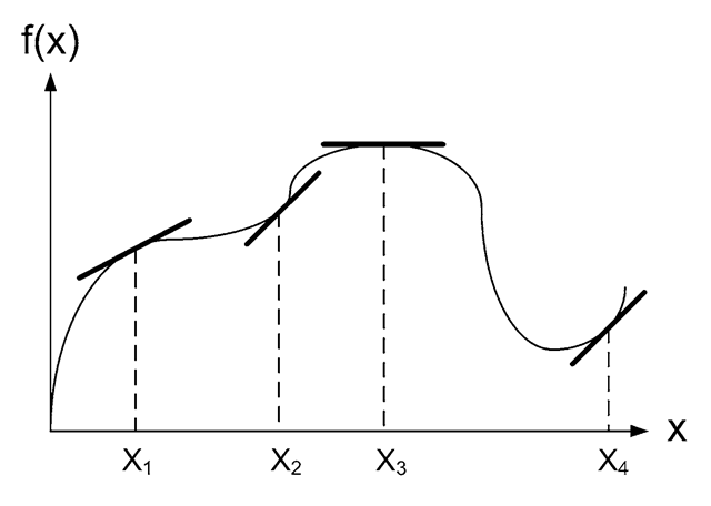
To enable edge detection we utilize the concept of gradients. We first present gradients for a general curve and then turn to gradients in images. In the 1D case we can define the gradient of a point as the slope of the curve at this point. Concretely this corresponds to the slope of the tangent at this point. In Fig. 5.12 the tangents of several different points are shown.

Fig. 5.12 A curve and the tangent at four points

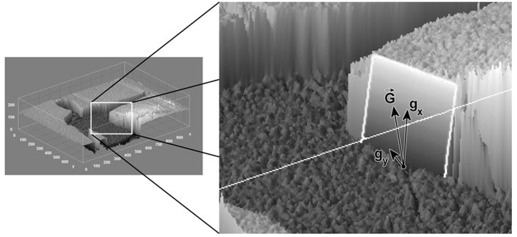
If we represent an image by height as opposed to intensity, see Fig. 5.13, then edges correspond to places where we have steep hills. For each point in this image landscape we have two gradients: one in the x-direction and one in the y-direction. Together these two gradients span a plane, known as the tangent plane, which intersects the point. The resulting gradient is defined as a vector ~G(gx,gy), where gx is the gradient in the x-direction and gy is the gradient in the y-direction. This resulting gradient lies in the tangent plane, see Fig. 5.14.

We can consider H(gx,gy) as the direction with the steepest slope (or least steepest slope depending on how we calculate it), or in other words, if you are standing at this position in the landscape you need to follow the opposite direction of the gradient in order to get down fastest. Or in yet another way, when water falls at this point it will run in the opposite direction of the gradient.

Fig.5 .13 A 3D representation of the image from Fig. 5.11, where the intensity of each pixel is interpreted as a height

Fig. 5.14 In a 3D representation of an image, a tangent plane is present for each point. Such a plane is defined by two gradient vectors in x- and y-direction, respectively. Here the tangent plane is shown for one pixel

Besides a direction the gradient also has a magnitude. The magnitude expresses how steep the landscape is in the direction of the gradient, or how fast the water will run away (if you go skiing you will know that the magnitude of the gradient usually defines the difficulty of the piste). The magnitude is the length of the gradient vector and calculated as

where the approximation is introduced to achieve a faster implementation.

Image Edges

For the curves shown above, the gradients are found as the first order derivatives denoted f ‘(x). This can only be calculated for continuous curves and since an image has a discrete representation (we only have pixel values at discrete positions: 0, 1, 2, 3, 4 etc.) we need an approximation. Recalling that the gradient is the slope at a point we can define the gradient as the difference between the previous and next value. Concretely we have the following image gradient approximations:

We have included (x, y) in the definition of the gradients to indicate that the gradient values depend on their spatial position. This approximation will produce positive gradient values when the pixels change from dark to bright and negative values when a reversed edge is present. This will of course be opposite if the signs  are switched, i.e.,1) – f(x, y + 1). Normally the order does not matter as we will see below.

Fig. 5.15 Prewitt and Sobel kernels

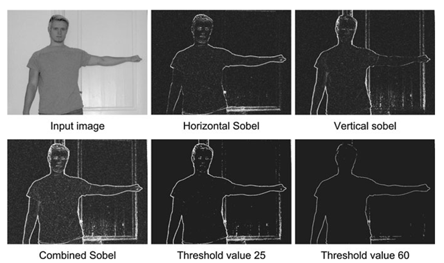
Fig. 5.16 Sobel kernels applied to an image. Each individual kernel finds edges that the other does not find. When they are combined a very nice resulting edge is created. Depending on the application, the threshold value can be manipulated to include or exclude the vaguely defined edges

Equation 5.10 is applied to each pixel in the input image. Concretely this is done using correlation. We correlate the image with a 1 x 3 kernel containing the following coefficients: -1,0, 1. Calculating the gradient using this kernel is often too sensitive to noise in the image and the neighbors are therefore often also included into the kernel. The most well know kernels for edge detection are illustrated in Fig. 5.15: the Prewitt kernels and the Sobel kernels. The difference is that the Sobel kernels weight the row and column pixels of the center pixel more than the rest.

Correlating the two Sobel kernels with the image in Fig. 5.11 yields the edge images in Fig. 5.16. The image to the left enhances horizontal edges, while the image to the right enhances vertical edges. To produce the final edge image we use Eq. 5.9.

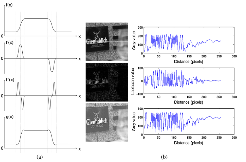
Fig. 5.17 (a) The principal behind image sharpening. (b) An example of image sharpening with c = 0.6. The pixel values of a horizontal line (the location is indicated by the white line in the top image) are shown to the right

That is, we first calculate the absolute value of each pixel in the two images and then add them together. The result is the final edge enhanced image. After this, the final task is often to binarize the image, so that edges are white and the rest is black. This is done by a standard thresholding algorithm. In Fig. 5.16 the final edge enhanced image is shown together with binary edge images obtained using different thresholds. The choice of threshold depends on the application.

Image Sharpening

The method presented in Sect. 4.4.2 and illustrated in Fig. 4.23 is not only applicable to thresholding, but can also be used to increase the overall contrast of the image. The method is expressed as follows in terms of correlation:

where h(x, y) is a large mean filter kernel. The method belongs to the class of methods aimed at sharpening or enhancing the image. Another method for this purpose is based on image edges and is explained in the following.

What makes it possible to see an object in a scene, is the fact that the object is different from the background. From this follows that the transition between object and background is of great importance and this is of course exactly why we measure edges in an image.

Fig. 5.18 Left: Kernels for approximating the second order derivatives. Right: Laplacian kernel

If we could somehow make the edges steeper the difference between object and background would be even more profound and hence the image sharper to look at. A way of doing this is shown in Fig. 5.17(a). The first figure shows the pixel values of an image row. x denotes the position in the row and f(x) is the gray-level value. The next figure shows the gradient value, or the first derivative f ‘(x), of f(x). The third figure is the second order derivative of f(x), denoted f " (x). It expresses the gradient of the gradient. What we can see is that g(x) = f(x) — c · f "(x) does exactly what we are interested in, namely to make the edges steeper. The constant c can be used to weight the amount of sharpness that is desired. For an image the second order derivatives can be approximated as

where gxx(x, y) and gyy(x, y) are the second order derivatives in the x- and y-direction, respectively. These two expressions can easily be expressed as kernels, see Fig. 5.18, and correlated with the image. However, instead of correlating with both kernels and combining the results, we can combine them into the joint kernel, h(x,y), and only do one correlation. This joint kernel is denoted the Laplacian kernel and shown below. Mathematically this image sharpening method is expressed as follows and illustrated in Fig. 5.17(b):

where c is a constant and h(x,y) is the Laplacian kernel. Note that for both Eqs. 5.12 and 5.15 an implementation needs to make sure the output image is mapped to [0, 255]. This can be done by the method in Sect. 4.6.

Further Information

Correlation is related to the term convolution and both are used throughout the video and image processing literature. Convolution only differs by the way the kernel is applied to the image beneath it. Mathematically convolution is defined as:

 

 

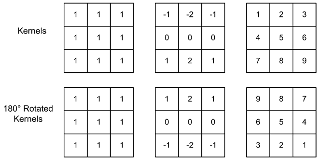
Fig. 5.19 Three kernels and their rotated counterparts

Comparing this to the equation for correlation in Eq. 5.4 we can see that the only differences are the two minus signs. The interpretation of these is that the kernel is rotated 180° before doing a correlation. In Fig. 5.19 examples of rotated kernels are shown. What we can see is that symmetric kernels are equal before and after rotation, and hence convolution and correlation produce the same result. Edge detection kernels are not symmetric. However, since we often only are interested in the absolute value of an edge the correlation and convolution again yield the same result.

When applying smoothing filters, finding edges etc. the process is often denoted convolution even though it is often implemented as correlation! When doing template matching it is virtually always denoted correlation.

One might rightfully ask why convolution is used in the first place. The answer is that from a general signal processing5 point of view we actually do convolution, and correlation is convolution done with a rotated kernel. However, since correlation is easier to explain and since it is most often what is done in practice, it has been presented as though it were the other way around in this (and many other) texts.

Edge detection is a key method in many image processing systems and a number of different methods have therefore been suggested over the years. Using the Sobel kernels works well, but results in wide edges as can bee seen in Fig. 5.17. If we are interested in knowing the exact edge, i.e., a 1-pixel thin edge, then the same figure suggests to use the second order derivatives and look for the places where the values change from positive to negative or vise versa. These places are denoted zero-crossings. As mentioned above the first order derivatives are sensitive to noise in the images. This problem is even more profound for the second order derivatives. The image is therefore smoothed using a Gaussian filter before the Laplacian is applied to approximate the second order derivatives and looking for zero-crossings.

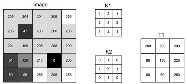
Fig. 5.20 K1 and K2 are kernels, while T1 is a template

Another approach to finding 1-pixel thin edges is the Canny edge detector [5]. It first smooths the image using a Gaussian filter before applying the Sobel kernels. From the Sobel kernels the direction of the gradient in each point is estimated. Next, the principle of non-maximum suppression is applied. For each pixel the magnitude of the gradient is compared with the magnitudes of the two nearest neighbors in the gradient direction. The two smallest are deleted. Applying this to all pixels results in 1-pixel thin edges. Finally a threshold is applied to prune edges with too small magnitudes. If, however, an edge with a too small magnitude is connected6 to a pixel with a magnitude above another threshold value, then the edge is not pruned. This allows for an adaptive pruning and is known as the principle of hysteresis thresholding.

Sometimes template matching is preformed on binary edge images. If the shape of the object in the image is slightly different from the input image, the template matching will output a very low similarity even though the two objects might look very similar. Therefore Chamfer matching [2] can be applied instead. Here the template image is converted into an image where each pixel contains a value indicating the distance to the nearest edge, see Sect. 6.4. Using such a distance-image as the template will provide a much more stable result.