Introduction
Urban features (e.g. roads, buildings) often have sharp boundaries. Because of the coarse spatial resolution of most remotely sensed images relative to such features, many pixels (particularly those containing boundaries) will contain a mixture of the spectral responses from the different features.These techniques are based on the assumption that the spectral value of each pixel is the composite spectral signature of the land cover types present within the pixel. For example, mixture modelling, neural networks and the fuzzy c-means classifier have been compared for predicting the proportions of different classes that a pixel may represent.While these ‘soft’ classifiers offer benefits over traditional ‘hard’ classifiers, no information is provided on the location of the land cover proportions within each pixel.
A per-field approach using detailed vector data can be used to increase the spatial resolution of the remote sensing classification and increase classification accuracy (Aplin et al., 1999a, 1999b). In most cases, however, accurate vector data sets are rarely available (Tatem et al., 2001). Therefore, it is important to consider techniques for sub-pixel mapping that do not depend on vector data.
A method was applied previously to map the sub-pixel location of the land cover proportions predicted from a mixture model based only on the spatial dependence (the likelihood that observations close together are more similar than those further apart) inherent in the data.The approach was based on maximizing the spatial dependence in the resulting image at the sub-pixel scale. However, the resulting spatial arrangement conflicted with our understanding of what constitutes ‘maximum spatial order’, as the author indicated.In an attempt to circumvent this problem, the proposed approach was designed to take account of contributions to the sub-pixel classification from both the centre of the ‘current’ pixel and from its neighbouring pixels. These ‘contributions’ are based on the assumption that the land cover is spatially dependent both within and between pixels.
Conventional classifiers such as the maximum likelihood classifier (MLC) are based on the spectral signatures of training pixels and do not recognize spatial patterns in the same way that a human interpreter does (Gong et al., 1990). However, the MLC generates a substantial amount of information on the class membership properties of a pixel, which provides valuable information on the relative similarity of a pixel to the defined classes.The objective of the proposed approach was to use such probability measures derived from the MLC together with spatial information at the pixel scale to produce a fine spatial resolution land cover classification (i.e. at the sub-pixel scale), potentially with increased accuracy. Therefore, in the proposed approach for sub-pixel mapping, two stages (spectral-spatial) were employed. In the first stage, a MLC is implemented and a posteriori probabilities are predicted. In the second stage, an inverse distance weighting predictor is used to interpolate a probability surface at the sub-pixel scale from the probabilities of the central pixel and its neighbourhood. Subsequently, a sub-pixel hard classification is produced based on the interpolated probabilities at the sub-pixel scale.
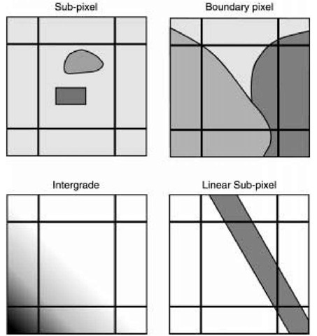
Among the four causes of mixed pixels described by Fisher, and shown in Figure 5.1 (Fisher, 1997), the ‘boundary pixel’ and ‘intergrade’ cases are investigated in this topic because they are the most amenable to sub-pixel analysis. The ‘sub-pixel’ and ‘linear sub-pixel’ cases are beyond the present scope because of the lack of information on the existence and spatial extent of objects smaller than the pixel size. Nevertheless, the proposed sub-pixel approach aims at solutions to the ‘boundary pixel’ and ‘intergrade’ cases without neglecting the potential existence of the other two cases.
Thus, the objective was to present a new method to produce a land cover classification map with finer spatial resolution than that of the original imagery, with potentially increased accuracy, especially for boundary pixels. The results will be used in later research to infer urban land use based on a land cover classification.
Methods
Sub-pixel classification
After implementing the standard MLC, the proportion of each class in a pixel was related to the pixel’s probability vector. Each pixel was split into 5 x 5 = 25 sub-pixels with a zoom factor of 5.
Figure 5.1 Four causes of mixed pixels.
This zoom factor was chosen to match the difference in the spatial resolutions of Systeme Pour L’Observation de la Terre (SPOT) High Resolution Visible (HRV) and IKONOS multispectral (MS) imagery, which are a focus of this topic. To determine the class probability of a sub-pixel for each class, a new probability vector z was calculated based on the probability vectors of the central pixel and its eight neighbouring pixels. The inverse distance weighting predictor was used in computing a new probability value for each sub-pixel. The assumption is that the value of an attribute z at an unvisited point is a distance-weighted average of data points occurring within a neighbourhood or window surrounding the unvisited point (Burrough and McDonnell, 1998).
where,![]() is the value of the attribute at an unvisited location
is the value of the attribute at an unvisited location![]() is the known value of the attribute at location
is the known value of the attribute at location![]() is the distance between the unknown point
is the distance between the unknown point ![]() and a neighbour
and a neighbour![]() is a distance weighting factor and n is the number of neighbours.
is a distance weighting factor and n is the number of neighbours.
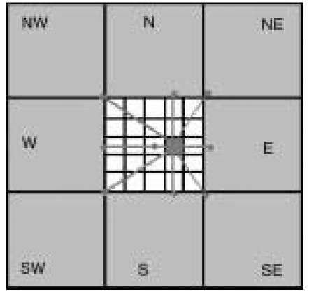
For a given sub-pixel the distances to the centres of the neighbours are calculated. These distance measures dj are used to calculate the new probability vector of the sub-pixel![]() see Figure 5.2 (sub-pixel-central). Another option is to take the distances from a given sub-pixel to the edges of the neighbours to the north, east, south and west and to the corners of the neighbours to the north-west, north-east, south-east and south-west (see Figure 5.3, sub-pixel-corner). The effect of these different distance measures on the interpolation result was tested. The distance weight exponent r was set to 1.0.
see Figure 5.2 (sub-pixel-central). Another option is to take the distances from a given sub-pixel to the edges of the neighbours to the north, east, south and west and to the corners of the neighbours to the north-west, north-east, south-east and south-west (see Figure 5.3, sub-pixel-corner). The effect of these different distance measures on the interpolation result was tested. The distance weight exponent r was set to 1.0.
Figure 5.2 Inverse distance interpolation used to compute sub-pixel probability vectors. Distances are taken from each sub-pixel to the centres of neighbouring pixels
Figure 5.3 Inverse distance interpolation used to compute sub-pixel probability vectors. Distances are taken from each sub-pixel to the corners or edges of neighbouring pixels
An important factor to consider is how to incorporate the probability vector of the current pixel itself into the interpolation. One option is to leave the centre probability vector out. In this case, only the neighbouring probability vectors would be used (to neglect the existence of the ‘sub-pixel’ and ‘linear sub-pixel’ cases in Figure 5.1). Another option is to choose a distance value for the centre probability pixel in the interpolation (e.g. to consider the potential existence of the ‘sub-pixel’ and ‘linear sub-pixel’ cases in Figure 5.1). For example, the distance from each sub-pixel to the centre pixel could be set to 1.0 to give this pixel a large weight.
Experimental testing
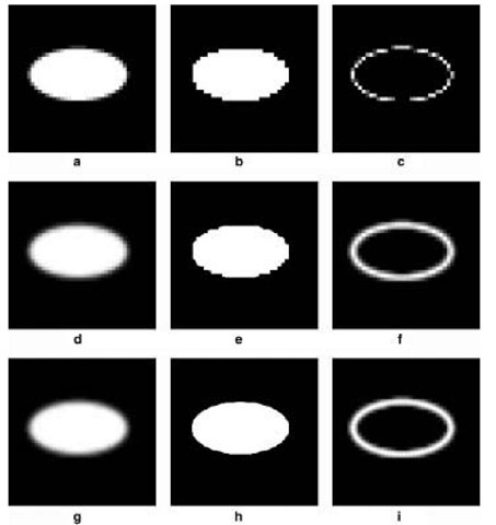
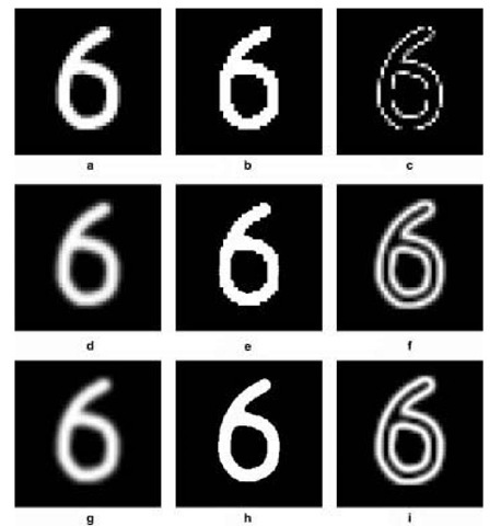
To assess the accuracy of the proposed sub-pixel approach, several controlled tests were implemented. Four binary testing images were created manually at the sub-pixel scale (200 x 200 pixels) with values of 1 and 0 (white and black respectively in Figure 5.4). Simulated probability images (40 x 40 pixels) were generated from four testing images by aggregating sub-pixels into pixels. Equal-weighted aggregation was used to maintain the statistical and spatial properties of the simulated data (Bian and Butler, 1999). Simulated images can be found in Figures 5.5(a), 5.6(a), 5.7(a) and 5.8(a) (40 x 40 pixels). Each pixel of a simulated image covers 5 x 5 sub-pixels corresponding to the same spatial aggregation scale of SPOT HRV imagery (20 m) relative to IKONOS MS imagery (4m).
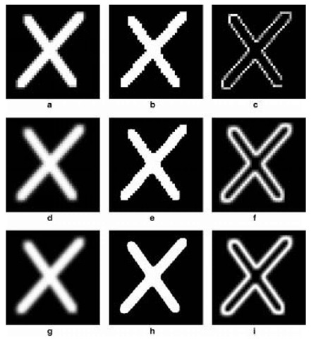
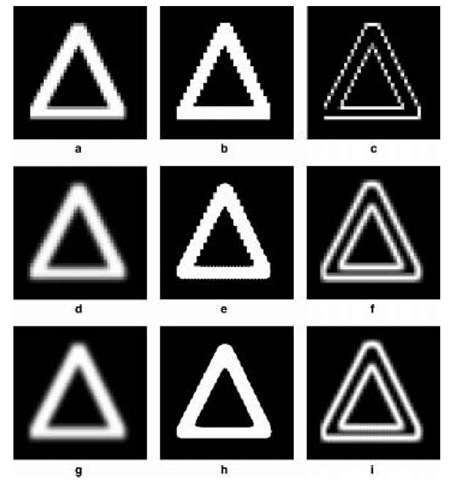
The above sub-pixel approaches were applied to the simulated images. Probability images were generated by applying the proposed interpolation method using the central points of neighbouring pixels (Figures 5.5(d), 5.6(d) 5.7(d) and 5.8(d)) and using the corners or edges of neighbouring pixels (Figures 5.5(g), 5.6(g), 5.7(g) and 5.8(g)) respectively. Corresponding outputs at the sub-pixel scale are shown in Figures 5.5(e), 5.6(e), 5.7(e) 5.8(e) and Figures 5.5(h), 5.6(h), 5.7(h) and 5.8(h) respectively.
Accuracy assessment
Accuracy assessment was carried out in the following three ways:
Figure 5.4 Experimental ‘truth’ images (200 x 200 pixels)
Figure 5.5 Experimental testing results based on the proposed sub-pixel interpolation method: (a) resampled image from experimental truth image (Figure 5.4a); (b) classification results based on resampled image; (c) entropy results of (b) (40 x 40 pixels); (d) probability image at the sub-pixel scale using central points of neighbouring pixels; (e)classification results at the sub-pixel scale based on (d); (f)entropy results of (e)(200 x 200 pixels); (g)probability image at the sub-pixel scale using the corners or edges of neighbouring pixels; (h) classification results at the sub-pixel scale based on (g); (i) entropy results of (h) (200 x 200 pixels)
Overall accuracy and producer’s accuracy
The accuracy of classification was estimated by comparing the classified data with the testing data on a pixel-by-pixel basis at the sub-pixel scale (each pixel of results at the pixel scale (b) in Figure 5.5 was split into 5 x 5 pixels at the sub-pixel scale). Overall accuracy was calculated as
Figure 5.6 Experimental testing results based on the proposed sub-pixel interpolation method: (a) resampled image from experimental truth image (Figure 5.4b); (b) classification results based on resampled image; (c) entropy results of (b) (40 x 40 pixels); (d) probability image at the sub-pixel scale using central points of neighbouring pixels; (e)classification results at the sub-pixel scale based on (d); (f)entropy results of (e) (200 x 200 pixels); (g) probability image at the sub-pixel scale using the corners or edges of neighbouring pixels; (h) classification results at the sub-pixel scale based on (g); (i) entropy results of (h) (200 x 200 pixels)
where,![]() __ is the number of pixels classified correctly, N is the total number of pixels and k is the number of classes. Producer’s accuracy was used to represent classification accuracy for individual classes:
__ is the number of pixels classified correctly, N is the total number of pixels and k is the number of classes. Producer’s accuracy was used to represent classification accuracy for individual classes:
Figure 5.7 Experimental testing results based on the proposed sub-pixel interpolation method: (a) resampled image from experimental truth image (Figure 5.4c); (b) classification results based on resampled image; (c) entropy results of (b) (40 x 40 pixels); (d) probability image at the sub-pixel scale using central points of neighbouring pixels; (e)classification results at the sub-pixel scale based on (d); (f)entropy results of (e); (200 x 200 pixels); (g)probability image at the sub-pixel scale using the corners or edges of neighbouring pixels; (h) classification results at the sub-pixel scale based on (g); (i) entropy results of (h) (200 x 200 pixels)
where,![]() is the number of pixels classified correctly,
is the number of pixels classified correctly,![]() is the number of pixels classified into class i in the testing data set and k is the number of classes.
is the number of pixels classified into class i in the testing data set and k is the number of classes.
Figure 5.8 Experimental testing results based on the proposed sub-pixel interpolation method: (a) resampled image from experimental truth image (Figure 5.4d); (b) classification results based on resampled image; (c) entropy results of (b) (40 x 40 pixels); (d) probability image at the sub-pixel scale using central points of neighbouring pixels; (e) classification results at the sub-pixel scale based on (d); (f) entropy results of (e) (200 x 200 pixels); (g) probability image at the sub-pixel scale using the corners or edges of neighbouring pixels; (h) classification results at the sub-pixel scale based on (g); (i) entropy results of (h) (200 x 200 pixels)
