Pixel Unmixing at the Sub-pixel Scale Based on Land Cover Class Probabilities: Application to Urban Areas Part 2

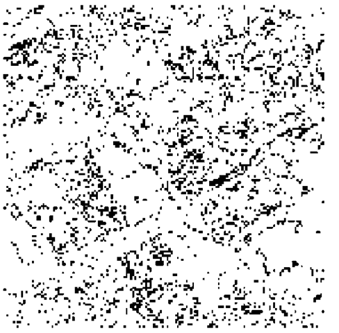
Kappa coefficient

Kappa analysis is a discrete multivariate technique used in accuracy assessment for determining statistically if one error matrix is significantly different from another (Bishop et al., 1975). The Kappa analysis has become a popular component of accuracy assessment (Hudson and Ramm, 1987; Congalton, 1991; Richards, 1993; Congalton and Green, 1999). The Kappa statistic is given by

where,is the number of pixels classified correctly,is the number of pixels classified into classis the number of pixels classified into class i in the testing data set, N is the total number of pixels and k is the number of classes.

Entropy

The accuracy of a classification may be indicated by the way in which the probability of class membership is partitioned between the classes and this may be expressed by entropy measures. Entropy, given by

where, Pi is the probability of belonging to class i, was used to further assess uncertainty in this topic.

The results are indicated (see also Table 5.1) for each case as overall accuracy, Kappa coefficient and entropy images in Figure 5.5(c), (f) and (i), respectively. Figure 5.5 shows that the results are promising for each case. The results show that both interpolation methods have the ability to increase classification accuracy and classify at a spatial resolution that is finer than that of the original data. It also shows that more accurate results have been produced by using the corner or edge points of neighbouring pixels than by using the central point of neighbouring pixels. Therefore, only the interpolation method using the corner or edge points of neighbouring pixels was applied in the following case study based on real imagery.

Study Area

A 9 km2 (3 km x 3 km) area, south-east of Amsterdam, was selected for the experiment. Approximately 200 000 people live in this sub-urban district. Several types of residential as well as commercial areas, parks, lakes and canals can be found in the study area. Built-up areas, green space and water are three constituent land cover classes in this study.

Table 5.1 Testing results using overall accuracy and Kappa coefficient

Test Image	Pixel Scale		Sub-pixel Scale using corners or edges		Sub-pixel Scale using central points
	Overall Accuracy	Kappa Coefficient	Overall Accuracy	Kappa Coefficient	Overall Accuracy	Kappa Coefficient
‘Cross’	97.85%	93.12%	98.22%	94.32%	99.24%	97.60%
‘Triangle’	97.26%	91.35%	97.98%	93.57%	99.39%	98.03%
‘Ellipse’	99.11%	97.06%	99.34%	97.80%	99.75%	99.16%
‘Six’	98.30%	92.49%	98.62%	93.93%	99.46%	97.61%

SPOT HRV imagery was used for urban land cover classification. A detailed land cover map was prepared for training and testing purposes based on detailed topographic maps (scale 1:1000) together with visual interpretation of IKONOS MS imagery (same 4 m pixel size as the final sub-pixel outputs) of the same area. The final results were analysed to determine the effectiveness of the use of posterior probabilities and the proposed sub-pixel approach to increase the accuracy of land-cover classification and to produce finer spatial resolution classification maps.

Applications

Data and sample selection

The data used in the case study are listed in Table 5.2.

To minimize the potential bias in the MLC, the single-pixel training approach was used in the sample selection. About 100 data for each class were selected manually from the SPOT HRV image following the rules discussed in the literature (Gong and Howarth, 1990).

Land cover classification using MLC

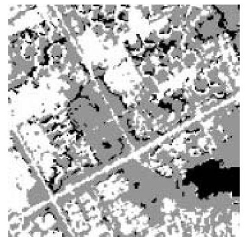
Land cover classification was implemented using a standard MLC algorithm (Richards, 1993). The classification results consisted of ‘hard’ classification output (Figure 5.9) and the probability map for each class.

Preparation of testing data

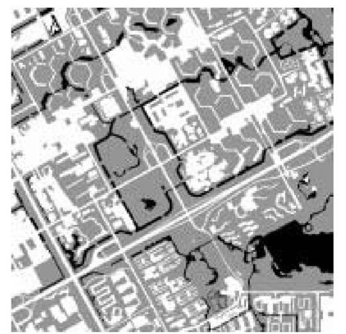
The training and testing data were prepared based on visual interpretation of IKONOS MS imagery and large-scale topographical maps (1:1000). Colour aerial photographs taken in 1996 and 1997 were used to simulate the situation in 1996 when SPOT HRV imagery was captured. The final map was produced by vector-to-raster conversion with a spatial resolution of 4m, the same as that of IKONOS MS imagery. Figure 5.10 shows the testing data used in the accuracy assessment.

Pixel unmixing

Pixel unmixing was implemented by a program developed by the authors in Java using the inverse distance weighting interpolation method based on corner or edge points of neighbouring pixels (section 2).

Table 5.2 List of data used in the experiments

Type of data	Sensor	Date	Band/Colour	Spatial resolution	Scale
Satellite sensor	SPOT	13 Oct. 1996	Multi-spectral	20m	N/A
imagery	IKONOS	8 June 2000	Multi-spectral	4m	N/A
Aerial	Optical	19 May 1997	True colour	N/A	1:10 000
photographs	camera	30 May 1999
Topographic		1996, 1997,	Black and	N/A	1:1000
maps		1999	white

Figure 5.9 Classification map produced by applying the standard MLC approach at the pixel scale (150 x 150 pixels)

Figure 5.10 Image prepared at the sub-pixel scale (750 x 750 pixels), used for both training and testing

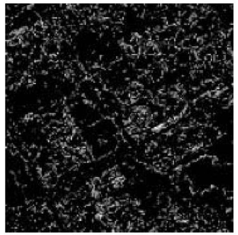
The sub-pixel classification results consist of ‘hard’ classification output (Figure 5.11) and the probability map for each class at the sub-pixel scale as well as the entropy map (Figure 5.12) based on the interpolated probability map for uncertainty assessment.

Accuracy assessment

Accuracy assessment was based on pixel-to-pixel comparison between produced classification results achieved by different approaches with the testing map at the sub-pixel scale.

Figure 5.11 Classification map produced by applying the sub-pixel approach at the sub-pixel scale (750 x 750 pixels)

Figure 5.12 Entropy map produced based on the interpolated probability map at the sub-pixel scale (750 x 750 pix els)

Table 5.3 Comparison of accuracies obtained by applying the standard MLC and the sub-pixel approach

Accuracy assessment	Standard MLC	Sub-pixel
Overall accuracy	73.66%	74.57%
Kappa	53.15%	54.00%

Each pixel of results (Figure 5.9) was split into 5 x 5 sub-pixels to enable a pixel-to-pixel comparison with the testing map at the sub-pixel scale. Overall accuracy and the Kappa coefficient are presented in Table 5.3. Producer’s accuracy was used to represent classification accuracy for individual land cover classes Table 5.4). An entropy map was produced based on the interpolated probability map at the sub-pixel scale (Figure 5.12).

Impacts of applying the sub-pixel approach to boundary pixels

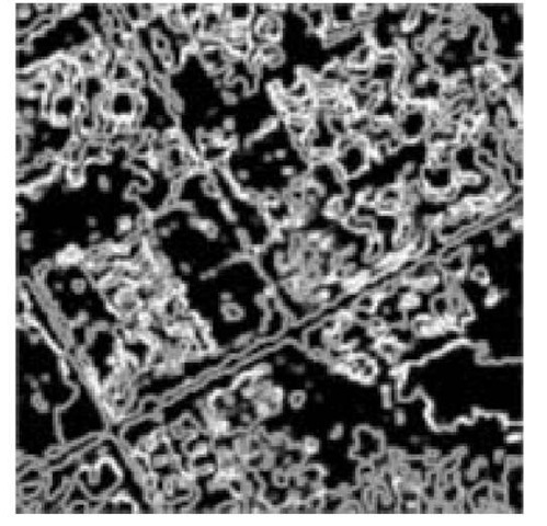
To assess the impacts of the proposed approach on boundary pixels (the main goal of this topic) in detail, the entropy map was produced based on the probability values to each class at the pixel scale (Figure 5.13). About 14% of the total number of pixels were extracted as boundary pixels (Figure 5.14) based on the entropy map (Figure 5.13) using a threshold value of 0.469. A threshold value of 0.469 means that no one class is dominant (maximum likelihood > 0.9) in comparing probabilities to each class (with three classes). Non-boundary pixels can be interpreted as having at least one class dominant among all classes.

Classification maps produced by applying the standard MLC and the sub-pixel approach were compared with the testing map using boundary pixels and non-boundary pixels as masks. The comparison results are shown in Tables 5.4 and 5.5.

Figure 5.13 Entropy map produced based on MLC probability at the pixel scale (150 x 150 pixels)

Figure 5.14 Boundary pixels (black) extracted from entropy map in Figure 5.13 (150 x 150 pix els)

Discussion

From Table 5.2, both overall accuracy and Kappa increased slightly (about 1%) using the proposed sub-pixel approach. Table 5.4 shows that the overall accuracy also increased by 4.58% for boundary cases for the sub-pixel approach.

The producer’s accuracy increased for the built-up area and green space, but decreased for water (Table 5.4). For boundary cases (Table 5.6), the producer’s accuracy increased for the built-up area and green space (6.09% and 7.36%). However, the producer’s accuracy decreased for water again (13%). When the classification map (Figure 5.11) is compared with the testing data map (Figure 5.10), it can be seen that some pixels along narrow canals had been eliminated by the sub-pixel approach.

Table 5.4 Comparison of producer’s accuracies obtained for each land cover class by applying the standard MLC and the sub-pixel approach

Land cover classes	Standard MLC	Sub-pixel
Built-up area	80.19%	80.99%
Green space	72.29%	74.01%
Water body	58.02%	53.61%

Table 5.5 Comparison of accuracies obtained by applying the standard MLC and the sub-pixel approach to boundary and non-boundary cases

Overall accuracy	Standard MLC	Sub-pixel
Boundary pixels	48.65%	53.23%
Non-boundary pixels	77.71%	78.03%

Table 5.6 Comparison of producer’s accuracies for land cover classes by applying standard MLC and the sub-pixel approach in boundary and non-boundary cases

Producer’s accuracy for land cover classes		Standard MLC	Sub-pixel
Boundary	Built-up area	44.98%	51.07%
pixels	Green space	50.22%	57.58%
	Water body	48.01%	35.01%
Non-boundary	Built-up area	84.44%	84.59%
pixels	Green space	76.13%	76.87%
	Water body	60.58%	58.36%

From the entropy map (Figure 5.12), it can be seen that these pixels along canals gained greater uncertainty as well. The main reason is that the proposed approach fails to tackle the ‘sub-pixel’ and ‘linear sub-pixel’ cases. Further, pixels in shadow areas are often mixed up with water pixels in spectral-feature space. However, it increases classification accuracy in the ‘boundary’ and ‘intergrade’ cases, which are the main objectives of this topic.

Based on the above results, it can be seen that the proposed sub-pixel approach has the ability to increase classification accuracy and produce a map at a finer spatial resolution than that of the original imagery, with objects consisting of at least four pixels or narrow linear objects at least two pixels wide, but certainly not with small objects of a single pixel or smaller. It may be possible to apply different interpolation settings to preserve small objects being eliminated in the proposed spatial allocation stage.

Conclusions

Pixel unmixing is an important issue especially for urban applications due to the fragmentary nature of urban features. The experiment shows that the posterior probability is useful in detecting mixed pixels as well as for spatial sub-pixel analysis. Additional efforts have to be made in dealing with pixels in shadow areas.

The results indicate that the proposed sub-pixel approach can be useful in increasing the spatial resolution and increasing overall classification accuracy, especially for class boundaries. Since the proposed sub-pixel approach consists of two independent stages, class components analysis and spatial allocation respectively, it is also suitable for pixel unmixing based on class components derived from other approaches.

The proposed sub-pixel approach tries to recognize the potential existence of features smaller than a pixel by using the value of the central pixel when spatially allocating class components according to their neighbouring pixels. However, the factors that contribute to producing the digital number (DN) of a remotely sensed image are complicated and interrelated (Fisher, 1997; Cracknell, 1998). Further improvements are needed to deal with such difficult pixel unmixing issues.