EVOLUTION OF THE ISOLUMINANCE CONTOURS MODEL
Visualization software applications were introduced to enable the sheer volume of data produced by computers worldwide to be viewed in picture form. Visualization makes it easier for the human visual system to pick up trends, patterns, and relationships in the data. The first wave of these applications typically generated simple two-dimensional line graphs, bar charts, and pie charts on expensive graphics workstations.
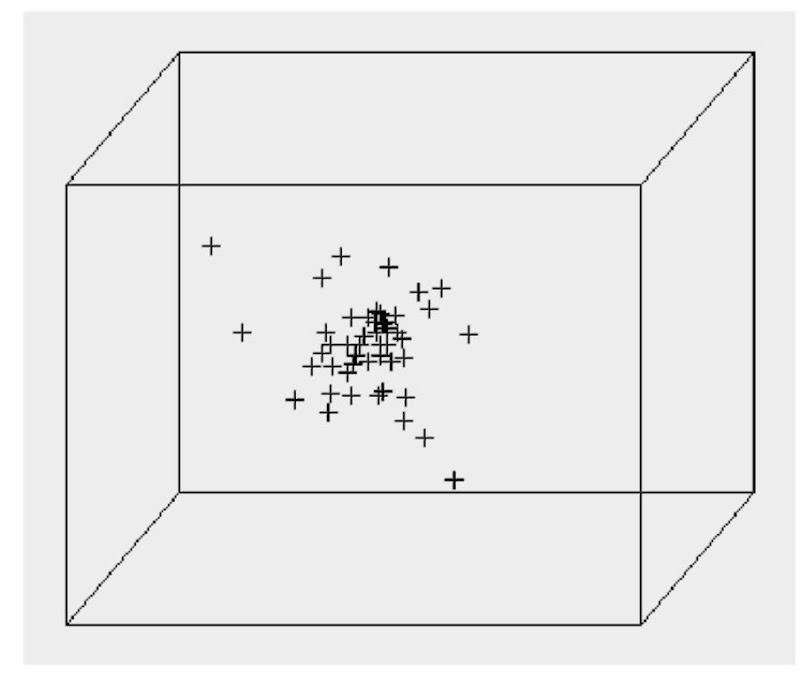
The second generation enabled three-dimensional images, with single data points typically denoted by dots or crosses, as shown in Figure 1. Axes lines or boxes enclosing the data were typically displayed. The whole image could then be rotated with the data points to give some indication of their orientation to each other. Since the majority of computers were not fast enough to perform the rotation in real-time, there was often some confusion in the picture’s interpretation.
Graphics software applications became available, such as OpenGL or DirectX, containing functions for creating simple solid objects such as cubes, cylinders, cones, and spheres, and researchers could now attempt their own visualization. Most of these graphical applications were based on the polyhedral representation and did not pro-vide any control over the number of patches representing each solid. Being able to animate the data points in realtime enhances trends and relationships in the data that are not easily identified in a still image. Since time is crucial in animation, representing solids with the minimum number of patches is of utmost importance.
Figure 1. Data cloud with data points denoted by crosses
The Isoluminance Contour model (IC model) was introduced in 1980 (Cottingham, 1981) as a means of representing these simple solids. It provides realistic results that far outweigh those produced using traditional methods, and in a fraction of the time. The amount of data used to generate an image can be easily adapted to suit each frame making real-time animation possible even on slow PCs.
Generating Images Using Traditional Graphics Techniques
Traditional graphics techniques adopt a divide-and-con-quer approach to rendering solid objects. Each solid’s surface is subdivided into planar patches that are generated one-by-one to produce the image while balancing speed with realism.
Storage Considerations
Each surface patch consists of four edges, each defined by two vertices specified in three-dimensional space. Topological information defines how edges and vertices are connected. Because surface patches from the simple solids form complete rows and columns, the topology can be implied by the order of storage using the Compressed Data Structure (CDS) (Cottingham, 1985; 1987).
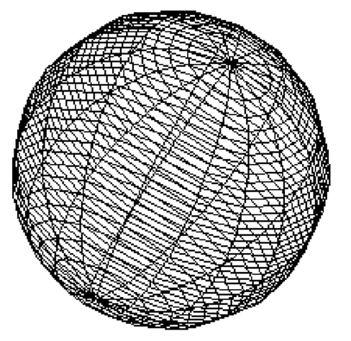
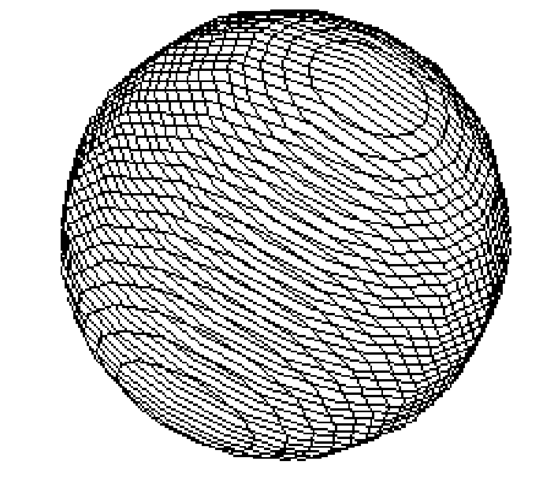
Figure 2 shows a sphere represented by 640 facets, stored in 41 rows of17 columns and generated by drawing lines to connect vertices stored at adjacent columns and rows. This is termed a wire frame drawing.
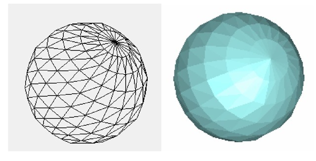
For speed, wire-frame drawings with only the edges of patches drawn are often used for quick previewing, but these do not provide much realism. At the next level, patches are flat shaded by calling a polygon fill function. However, in general, only triangular surfaces patches are guaranteed to be planar, so it is common practice for surface patches to be triangulated in an attempt to improve the degree of realism—this doubles the number of patches. Figure 3 shows a sphere defined by 11 rows and 21 columns of vertices that specify 400 triangular patches or 400 quadrilateral patches.
Figure 2. Wire-frame sphere
Isoluminance Contour Model (IC Model)
The Isoluminance Contour (IC) model takes an entirely different approach by representing solids by planar contours that are defined by a collection of perimeter points. Points that share the same orientation to the light source are chosen, therefore, they all share the same constant chromaticity. To generate a contour, the illumination model needs to be called only once before calling a polygon fill function. Contours are rendered in depth order. For speed, you can also simply apply linearly spaced chromaticity values without calling an illumination model at all and select one that achieves the required effect.
Using the Isoluminance Contour model, each contour is defined by a single row of vertices from the CDS array, so there is no need to connect vertices from adjoining rows. Figure 4 shows the planar contours drawn as a wire-frame image and Figure 5 shows the planar contours filled with color.
Using the IC model, hidden surface elimination is automatically performed by generating contours in depth order (Painter’s algorithm). The illumination model can be minimized to deciding on a range of color values and evaluating a contour’s color according to its distance from the light source. For optimum realism, a complex illumination model can be applied. This would achieve results indistinguishable to those produced using ray casting. Ray casting is considered to give the highest degree of realism of all the traditional rendering techniques available. It generates images pixel by pixel and is renowned for the vast amounts of CPU time it consumes. However, the Isoluminance Contour Model produces identical results, give or take a pixel, yet can produce images in a fraction of the time taken to produce even wireframe.
Comparison of Image Generation Speeds
Table 1 compares the CPU cycles taken to perform a single image containing a thousand spheres using traditional rendering methods on polyhedra with equivalent images produced using the IC model. For this comparison, each sphere was defined by 1250 patches—25 circular planes defined by 50 vertices, and the image was generated on a slow Pentium 400 PC. Although different hardware configurations will yield different results, the relative proportions of these times will remain constant.
For wire-frame drawings, all the edges for the polyhedral representation were drawn, displaying mainly quadrilateral patches; the IC model displays circular planes and avoids drawing the edges connecting the poles, as shown in Figure 4.
Figure 3. Flat-shaded sphere represented by triangulated patches
Figure 4. Isoluminance contour represents a sphere by a collection of planar contours
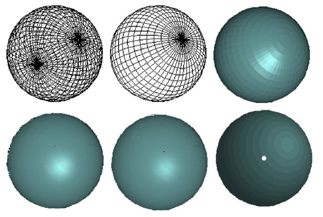
Different traditional techniques were applied to render the shaded images, each producing different levels of realism. The IC model used in the flat-shading timing included the specular reflection calculation, which is an add-on when required rather than part of the illumination model. The specular area shown in Figure 6 is the circular umbra that would appear if the light source was at the same angle as the viewing direction; this becomes more elliptical as the light is moved around. A higher level of realism would also require the penumbra to be displayed.
Using the IC model, a realistic image can be produced faster than even the simplest wire-frame image can be rendered by traditional methods. One reason is that only one normal and illumination calculation is required by the IC model for each ofthe 25 circular planes. In comparison, shading the polyhedral representation requires calculating the normals and illumination values for each of the 1250 vertices. In addition, when Gouraud’s smooth-shading method (1971) is used, these illumination values have to be interpolated at every pixel lying inside each patch. The slowest time used Phong’s (1975) method that requires the normals for every vertex to be interpolated and the illumination values calculated at every pixel lying inside each patch.
Figure 5. Filled isoluminance contours
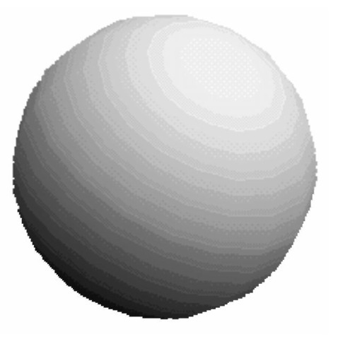
Figure 6 shows the images of one of the spheres rendered for this timing comparison. The top three spheres all use the polyhedral representation. From left to right, the polygons were rendered to produce a full wire-frame drawing, a wire-frame drawing with hidden lines re-moved, and a flat-shaded image. The bottom three spheres, from left to right, were rendered using Gouraud’s method and Phong’s method—both of which smooth-shaded patches from the polyhedra representation, and the IC model with specular reflection.
Figure 6. Spheres generated during the timing stage
Table 1. CPU times required to render a thousand spheres
| Full Wire frame | Wire Frame Hidden lines removed | Shaded | ||||
| Flat | Triangulated | Gouraud | Phong | |||
| Polyhedra | 9.33 | 222 | 238 | 262 | 313 | 1388 |
| IC model | 5.08 | 5.13 | 8.07 | - | - | - |
IC Model for Animated Visualization
Two approaches can be taken when animating data. In the first approach, the data points themselves are translated in three dimensions or rotated around one of the coordinate axes or about a line in three-dimensional space. In the second approach, the viewer moves around inside the data cloud and the data points remain static.
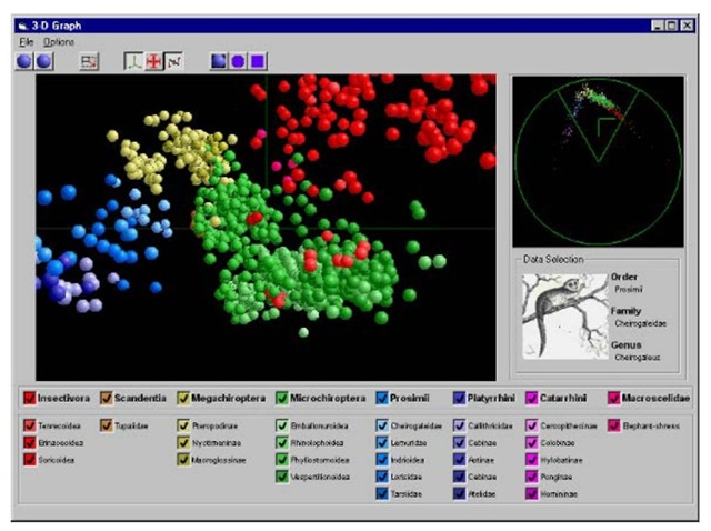
Figure 7 shows the three-dimensional visualization of the data points shown in Figure 1. These represent the evolution of mammals’ brains in terms of changes in overall brain size. This data set was supplied courtesy of Professor Heinz Stephan, Max-Planck Institut fur Hirmforschung, Frankfurt. Exploratory univariate and multivariate analyses were applied by Mr. Willem De Winter and Professor Charles Oxnard (Department of Anatomy and Human Biology at The University of Western Australia) to the volumes of11 non-overlapping brain parts from 921 specimens representing 363 species of various taxonomic groups consisting of primates, insec-tivores, bats, tree-shrews, and elephant shrews. This screen shot is from a visualization performed by software developed by Paul Merendah as an undergraduate, third-year Computer Graphics unit assignment (School of Computer Science and Software Engineering, The University of Western Australia). The assignment was specified and supervised by the author.
Uniform-sized spheres represent specimens, with the distances between the spheres representing the relative similarities in brain proportions (three dimensions). Perspective projection dictates the screen size of spheres. Species groups are color-coded (fourth dimension), and different levels of saturation and hue define individual relative significance within their animal group (fifth and sixth dimensions).
Figure 7. Visualization of the proportional sizes of the major brain divisions for a wide range of mammals
Figure 8. Visualization of the major brain divisions of mammals with different parameters in the illumination model
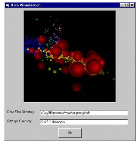
The data set contained 921 data points (spheres), and with the IC model it was possible to fly around the data cloud in real-time on a Pentium 166 PC. The relative position of the light source to the viewing position was assumed to be constant so that the contours of the spheres did not require reconstruction at any time during the simulation.
Figure 8 shows the same data set being visualized by software developed by Graham Wycherly in the same project; this software uses a different illumination model.
The ability to fly around the data clouds in real-time on such a slow PC was due to the adaptability of the IC model. The number of contours used for rendering any sphere was based on its screen size. The animation performed in these two student projects enabled even more relationships to be discovered, as before this dynamic visualization it was thought by biologists that the evolution of the brain in mammals was simply a matter of changes in the overall brain size (Finlay & Darlington, 1995). This visualization demonstrated the existence of different phylogenetic trends in the evolution of the mammalian brain and that where species shared a particular lifestyle the brain had evolved converging towards a similar proportional organization (Oxnard and de Winter 1997: 2journals, de Winter).
Both these projects assumed that the light source was positioned infinitely far away so that all light rays were parallel and all spheres were shaded the same. However, it is possible to remove this assumption and still attain real-time animation if you have a sufficiently powerful PC.
Allowing the position of the light source and the viewing position to move independently means that the light direction vector is no longer constant throughout the scene, therefore, the spheres at different positions in space no longer have identical shading. This makes it necessary to create each sphere from scratch whenever the viewing position or the light source changes. This is still achievable in real-time on a Pentium 400 or faster PC.
Figure 9. Light source positioned in the data cloud in full view of the viewing position
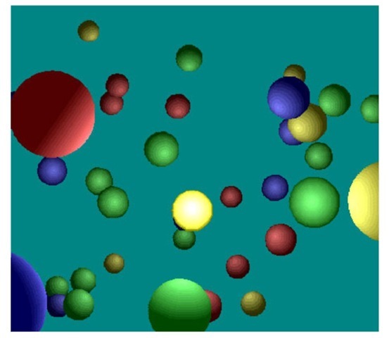
This independence means that the light source itself may become visible. Figure 9 shows the light source (brightest sphere) positioned amongst the data cloud in full view of the viewing position.
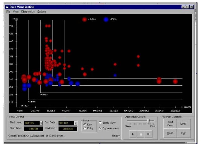
You may be required to display a timed series of data points on the screen simultaneously. The visualization shown in Figure 10 displays “bid and ask” stock market data over a five-day period. Professor Philip Brown from the Department of Accounting and Finance at The University of Western Australia supplied the data. The software was developed by Ken Hooi for a third-year Computer Graphics unit assignment that was specified and supervised by the author.
“Asks” are shares for sale at a specified price and “bids” are offers to buy at a stated bidding price. The asking price is usually more than the bidding price. The bids are displayed as blue spheres and asks as red spheres. The software creates an x- and y-axes pair for each day requested by the user and displays the bids and asks not realized for that day. The x-axis depicts the volume of the bid or ask parcels of shares, and the y-axis depicts the bid or ask price per share. When an ask parcel and a bid parcel match in price and volume then a transaction takes place and the relevant spheres disappear off the screen. The dynamic view allows the user to watch while the bid and ask pairs are being processed, so that he/she can view the trades as they happen.
IC Model as an Adaptive Model for RealTime Animation
Solids are created from templates to avoid having to recalculate the vertices for each one individually. To maintain the level of realism required, a template is defined by enough vertices to render the solid at its largest screen size. Since it would be inefficient to include all these vertices as the solid’s screen size diminishes, the number of vertices copied from the sphere template is adapted to reflect the screen area. For example, suppose the viewing position starts close to a sphere solid and moves away, causing the sphere to zoom away into the distance. Initially, all the vertices must be rendered to maximize the smoothness of the sphere’s surface. As the sphere moves away and its screen size grows smaller, every second vertex from every second contour can be used, then every third vertex from every third contour, and so on. For sphere solids, the screen size is calculated from the sphere’s diameter, which is approximated by (maximum X – minimum X).
Additional information on the IC model is available from Cottingham (1989, 2004a, 2004b), Cottingham and Conway (1988), and Conway (1991, 1993).
FUTURE TRENDS
First, the Isoluminance Contour model could be generalized by introducing a pre-processing step that takes existing data sets and combines any adjoining patches that have similar normal direction vectors. This would require a more general data structure such as Baumgart’s (1975)Winged-Edge Data Structure rather than the simpler CDS.
Second, because of the simplistic nature of the IC model, implementing it in hardware should be reasonably straightforward.
Figure 10. Displaying “bid and ask” stock market data one day per axis
CONCLUSION
The IC model is quick and simple to program as the topology of the solids is implied by the order of storage in a simple two-dimensional array. It eliminates the need for most of the steps required by traditional computer graphics techniques. It is extremely fast and does not require any quick-previewing methods to be developed. The realistic results that are indistinguishable from ray-tracing speak for themselves.
KEY TERMS
Data Cloud: Collection of data points in space.
Illumination Model: A mathematical formula for calculating the amount of diffuse light, ambient light, and specular reflection that contributes to the color value that will represent a particular surface point on the screen.
Isoluminance Contour: Planar polygon that has a single constant color at all points it encloses.
Real-Time Animation: Frames created at a minimum rate of 20 per second to avoid flicker.
Smooth-Shading Techniques: Interpolative techniques that restore the smoothness of solids whose surfaces are represented by planar polygons.
Viewing Position: The point in three-dimensional space where the user is positioned to view the data. There is also an associated direction where the user is looking.
Visualization: Viewing data in picture form in an attempt to gain a further understanding of the trends and relationships it contains.
Wire-Frame Drawing: Only the lines defining the edges of patches are drawn, which is useful as a quick previewing tool.
