INTRODUCTION
The traditional approach to forecasting involves choosing the forecasting method judged most appropriate of the available methods and applying it to some specific situations. The choice of a method depends upon the characteristics of the series and the type of application. The rationale behind such an approach is the notion that a “best” method exists and can be identified. Further that the “best” method for the past will continue to be the best for the future. An alternative to the traditional approach is to aggregate information from different forecasting methods by aggregating forecasts. This eliminates the problem of having to select a single method and rely exclusively on its forecasts.
Considerable literature has accumulated over the years regarding the combination of forecasts. The primary conclusion of this line of research is that combining multiple forecasts leads to increased forecast accuracy. This has been the result whether the forecasts are judgmental or statistical, econometric or extrapolation. Furthermore, in many cases one can make dramatic performance improvements by simply averaging the forecasts.
BACKGROUND OF COMBINATION OF FORECASTS
The concept of combining forecasts started with the seminal work 35 years ago of Bates and Granger (1969). Given two individual forecasts of a time series, Bates and Granger (1969) demonstrated that a suitable linear combination of the two forecasts may result in a better forecast than the two original ones, in the sense of a smaller error variance. Table 1 shows an example in which two individual forecasts (1 and 2) and their arithmetic mean (combined forecast) were used to forecast 12 monthly data of a certain time series (actual data).
The forecast errors (i.e., actual value – forecast value) and the variances of errors are shown in Table 2.
From Table 2, it can be seen that the error variance of individual forecast 1, individual forecast 2, and the combined forecast are 196, 188 and 150, respectively. This shows that the error variance of the combined forecast is smaller than any one of the individual forecasts and hence demonstrates an example how combined forecast may work better than its constituent forecasts.
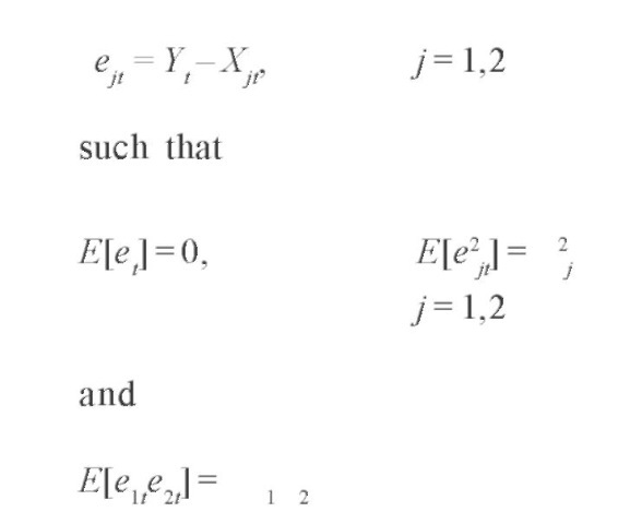
Bates and Granger (1969) also illustrated the theoretical base of combination of forecasts. Let Xlt and X2tbe two individual forecasts of Yt at time t with errors:
Table 1. Individual and combined forecasts
| Actual Data | Individual | Individual | Combined Forecast |
| (Monthly Data) | Forecast | Forecast | (Simple Average of |
| 1 | 2 | Forecast 1 and Forecast 2) | |
| 196 | 195 | 199 | 197 |
| 196 | 190 | 206 | 198 |
| 236 | 218 | 212 | 215 |
| 235 | 217 | 213 | 215 |
| 229 | 226 | 238 | 232 |
| 243 | 260 | 265 | 262.5 |
| 264 | 288 | 254 | 271 |
| 272 | 288 | 270 | 279 |
| 237 | 249 | 248 | 248.5 |
| 211 | 220 | 221 | 220.5 |
| 180 | 192 | 192 | 192 |
| 201 | 214 | 208 | 211 |

where 2. is the error variance of the individual forecast and is the correlation coefficient between the errors in the first set of forecasts and those in the second set.
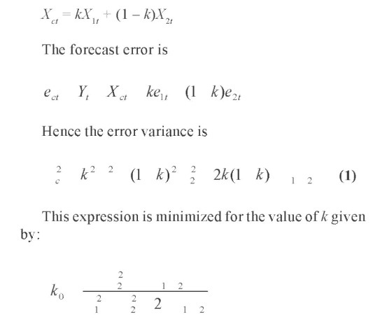
Consider now a combined forecast, taken to be a weighted average of the two individual forecasts:

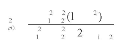
and substitution into equation (1) yields the minimum achievable error variance as:

Note that c20 < min( 2, 22) unless either is exactly equal to 1/ 2 or 2/ 1. If either equality holds, then the variance of the combined forecast is equal to the smaller of the two error variances. Thus, a priori, it is reasonable to expect in most practical situations that the best available combined forecast will outperform the better individual forecast—it cannot, in any case, do worse.
New bold and Granger (1974), Makridakis et al. (1982), Makridakis and Winkler (1983), Winkler and Makridakis (1983), and Makridakis and Hibbon (2000) have also reported empirical results that showed that combinations of forecasts outperformed individual methods.
Since Bates and Granger (1969), there have been numerous methods proposed in the literature for combining forecasts. However, the performance of different methods of combining forecasts varies from case to case. There is still neither definitive nor generally accepted conclusion that sophisticated methods work better than simple ones, including simple averages. As Clemen (1989) commented: In many studies, the average of the individual forecasts has performed the best or almost best. Others would agree with the comment of Bunn (1985) that the Newbold and Granger (1974) study and that of Winkler and Makridakis (1983) “demonstrated that an overall policy of combining forecasts was an efficient one and that if an automatic forecasting system were required, for example, for inventory planning, then a linear combination using a ‘moving-window’ estimator would appear to be the best overall”.
Table 2. Forecast errors and variances of errors
| Errors of Individual | Errors of Individual | Errors of Combined |
| Forecast 1 | Forecast 2 | Forecast |
| 1 | -3 | -1 |
| 6 | -10 | -2 |
| 18 | 24 | 21 |
| 18 | 22 | 20 |
| 3 | -9 | -3 |
| -17 | -22 | -19.5 |
| -24 | 10 | -7 |
| -16 | 2 | -7 |
| -12 | -11 | -11.5 |
| -9 | -10 | -9.5 |
| -12 | -12 | -12 |
| -13 | -7 | -10 |
| Variance of | Variance of errors = | Variance of |
| errors = 196 | 188 | errors = 150 |
DATA MINING AND COMBINATION OF FORECASTS IN INVENTORY MANAGEMENT
Data mining is the process of selection, exploration, and modeling of large quantities of data to discover regularities or relations that are, at first, unknown with the aim of obtaining clear and useful results for the owner of the database.
The data mining process is deemed necessary in a forecasting system, and it is particularly important in combining forecasts for inventory demands. Errors in forecasting demand can have a significant impact on the costs of operating and the customer service provided by an inventory management system. It is therefore important to make the errors as small as possible. The usual practice in deciding which system to use is to evaluate alternative forecasting methods over past data and select the best. However, there may have been changes in the process, generating the demand for an item over the past period used in the evaluation analysis. The methods evaluated may differ in their relative performance over sub-periods of the method that was best only part of the time, or in fact never the best method and perhaps only generally second best. Each method evaluated may be modeling a different aspect of the underlying process generating demands. The methods discarded in the selection process may contain some useful independent information. A combined forecast from two or more methods might improve upon the best individual forecasts. Furthermore, the inventory manager typically has to order and stock hundreds or thousands of different items. Given the practical difficulty of finding the best method for every individual item, the general approach is to find the best single compromise method over a sample of items, unless there are obvious simple ways of classifying the items, by item value or average demand per year, and so forth. Even if this is possible, there will still be many items in each distinct category for which the same forecasting method will be used. All of the points made on dealing an individual data series, as previously noted, apply with even more force when dealing with a group of items. If no one individual forecasting method is best for all items, then some system of combining two or more forecasts would seem a priori an obvious approach, if the inventory manager is going to use the same forecasting system for all items.
The need for data mining in combining forecasts for inventory demands comes from the selection of sample items on which forecasting strategy can be made for all items, the selection of constituent forecasts to be combined and the selection of weighting method for the combination.
The selection of the sample items is a process of exploratory data analysis. In this process, summary statistics such as mean and coefficient of variation can be investigated so that the sample selected could represent the total set of data series on inventory demands.
The selection of constituent forecasts to be combined is the first stage of model building. The forecasts methods might be selected from popular time series procedures such as exponential smoothing, Box-Jenkins and regression over time. One could include only one method from each procedure in the linear combination as the three groups of methods were different classes of forecasting model and thus might contribute something distinct, while there was likely to be much less extra contribution from different methods within the same class. It might also be useful to attempt to tailor the choice of methods to particular situations. For example, Lewandowski’s FORSYS system, in the M-competition (Makridakis et al., 1982), appears to be particularly valuable for long forecast horizons. Thus it might be a prime candidate for inclusion in situations with long horizons but not necessarily in situations with short horizons. It is also important to note that combining forecasts is not confined to combination utilizing time series methods. The desire to consider any and all available information means that forecasts from different types of sources should be considered. For example, one could combine forecasts from time series methods with forecasts from econometric models and with subjective forecasts from experts.
The second stage of model building is to select the weighting method for the combination of forecasts. The weighting method could be simple average or “optimal” weighting estimated by a certain approach, for instance, the constrained OLS method (Chan, Kingsman, & Wong, 1999b). Furthermore, the “optimal” weights obtained could either be fixed for a number of periods (fixed weighting) or re-estimated every period (rolling window weighting) (Chan, Kingsman, & Wong, 1999a, 2004). The selection process can then be done by comparing the different weighting methods with an appropriate performance measure. In the case of inventory management, the carrying of safety stocks is to guard against the uncertainties and variations in demand and the forecasting of demand. These safety stocks are directly related, or made directly proportional, to the standard errors of forecasts. If, as is usually the case, a stock controller is dealing with many items, it is the performance across the group of items that matters. Hence, the sum of the standard errors of the forecasts, measured by the sum of the root mean squared errors over all the items, can be used to compare the results between the different weighting methods. The ultimate aim is to find the one best overall method for the weighting process to use for all the items.
FUTURE TRENDS AND CONCLUSION
The usual approach in practical inventory management is to evaluate alternative forecasting methods over a sample of items and then select the one that gives the lowest errors for a majority of the items in the sample to use for all items being stocked. The methods discarded in the selection process may contain some useful independent information. A combined forecast from two or more methods might improve upon the best individual forecasts. This gives us some insights in the process of data mining. There are a number of well-known methods in data mining such as clustering, classification, decision trees, neural networks, and so forth. Finding a good individual method from our tool kit to handle the data is clearly an important initial step in data mining. Then we should always bear in mind the power in combining the individual methods. There are two kinds of direction to do the combination. The first one is basically a direct combination of the individual methods, such as simple average or “optimal” weighting. The other one is to classify our data first, and then select the weighting method. Classification is always an important aspect of data mining and combination of forecasts sheds some new light on this. Another important message is that if we are dealing with large data sets, then it is not very worthwhile to find the “best” individual method. Obviously, there may not be any best individual at all. A viable alternative is to find several sensible individual methods and then combine them as the final method. This approach will usually relieve much of our effort in finding the best individual method, as justified by the law of diminishing return.
KEY TERMS
Combination of Forecasts: Combine two or more individual forecasts to form a composite one.
Constrained OLS Method: A method to estimate the “optimal” weights for combination of forecasts by minimizing the sum of squared errors as in a regression framework, and the weights are constrained to sum to one.
Data Mining: The process of selection, exploration, and modeling of large quantities of data to discover regularities or relations that are at first unknown with the aim of obtaining clear and useful results for the owner of the database.
Fixed Weighting: “Optimal” weights are estimated and are used unchanged to combine forecasts for a number of periods.
Highest Weighting: Use the individual forecast procedure that is given the highest weight in the fixed weighting method. This is not a combination. This method is equivalent to choosing the forecasting technique which is the best on the weight estimation period.
Rolling Window Weighting: “Optimal” weights are estimated in each period by minimizing the errors over the preceding m periods, where m is the length in periods of the “rolling window”. The weights are then used to combine forecasts for the present period.
Simple Average Weighting: A simple linear average of the forecasts, implying equal weights for combination of forecasts.
