In This Chapter
Understanding the structure of an Excel database
Figuring out how criteria work
Adding, averaging, and counting database records
Finding the highest and lowest values
Testing for duplicate records
Creating sophisticated queries
Believe it or not, an Excel worksheet has the same structure as a database table. A database table has fields and records; an Excel worksheet has columns and rows. Same thing. Given this fact, why not ask questions of, or query, your information in much the same way as is done with a database?
In this chapter, we tell you how to use Excel’s database functions to get quick answers from sizeable lists of information. Let’s say for example, you had a client list on a worksheet — name, address, that sort of thing. You want to know how many clients are in New York. You may think about sorting your list by state and then counting the number of rows. Forget it — that’s the old way! In this chapter, we show you how to do this sort of thing with a single function.
Putting Your Data into a Database Structure
In order to use the database functions, you need to put your data into a structured format. Excel is very flexible. Usually, you put data wherever you want.
But to make the best of the database functions, you need to get your data into a contiguous area of rows and columns.
Figure 17-1 shows a database on a worksheet. This example is a list of students (by ID number), and the class, teacher, and grade for each student. Each student occupies a row in the database. There are four fields: Student ID, Class, Teacher, and Final Grade. Each field is in one column.
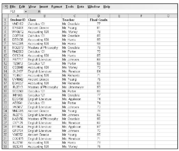
Figure 17-1:
Using a database to store student information.
The data on the worksheet in Figure 17-1 is really just normal data. There is nothing special about it. However, the data sits in organized rows and columns, making it ready for working with Excel’s database functions:
Each column is a field that holds one particular item of data, such as Student ID or Class. It must contain no other data.
Each row is a field that contains one record. In this example, a record is the data for one student.
The top row of the database contains labels that identify the fields.
This sample data is used to describe the database functions.
Understanding How the Database Functions Work
The database functions all follow the same format. These functions all use the following three arguments:
The database range: This argument tells the function where the database is. You enter it using cell addresses (for example, A1:D200) or a named range (for example, Students).
The field: You must tell a database function which field to operate on. You can’t expect it to figure this out by itself! You can enter either the column number or the field heading. A column number, if used, is the number of the column offset from the first column of the database area. In other words, if a database starts in Column C, and the field is in Column E, the column number is 3, not 5.If a heading is used, put it inside a set of double quotation marks. Database functions calculate a result based on the values in this field. Just how many values are used depends on the third argument — the criteria.
The criteria: This tells the function where the criteria are located. The criteria tell the function which records to use. The criteria are set up in a separate part of the worksheet that is not part of the database area, and you include the criteria range for this argument. Criteria use a heading and a value. The heading is the same as a field name, and a particular value goes underneath the heading. You can use an empty value to get a database function to operate on all the records in the database. We show you in more detail how criteria work throughout the chapter.
Establishing your database
All database functions take a database reference as the first argument. The database area must include headers (field names) in the first row. In Figure 17-1, the first row uses Student ID, Class, Teacher, and Final Grade as headers to the information in each respective column.
A great way to work with the database functions is to give the database area a name. Then you enter the name into the function instead of the range address. To set up a name, follow these steps:
1. Select the database area.
Make sure the top row has headers and is included in the selection.
2. Choose Insert O Name O Define.
The Define Name dialog box appears. The dialog box will already have the range set in the Refers To box.
3. Type a name in the top box (or use the suggested name).
4. Click OK to close the dialog box.
Later, if records are added to the bottom of the database, the range of the named area will have to be redefined. You can do this by going back into the Define Name dialog box and adjusting the reference. Here’s how:
1. Choose Insert O Name O Define to open the Define Name dialog box.
2. Click the named area in the Names in Workbook list.
Figure 17-2 shows an example of the Database_Area named area selected.
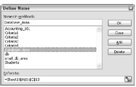
Figure 17-2:
Updating the reference to a named area.
3. Change the reference in the Refers To box.
You can use the small square button to the right of the Refers to box to define the new reference by dragging the mouse pointer over it. Clicking the small square button reduces the size of the Define Name dialog box and allows you access to the worksheet. When you are done dragging the mouse over the new worksheet area, press Enter to get back to the Define Name dialog box.
4. Click the OK button to save the reference change and close the dialog box.
Establishing the criteria area
The database functions look to an area of the worksheet that you specify to be the criteria. The criteria area can contain one or more individual criterion; each individual criterion is structured as follows:
In one cell, enter the field name (header) of the database column that the criterion will be for.
In the cell below, enter the value that the field data must meet.
Figure 17-3 shows the student database with a criteria area to the right of the database. There are places to put criterion for the Class, Teacher, and Final Grade. In the example, criterion has been set for the Class. The criterion will force the database function to only process records (rows) where the Class is Accounting 101. Note, though, that a criterion can be set for more than one field. In this example, the Teacher and Final Grade criteria have been left blank so they don’t affect the results.
The DAVERAGE function has been entered into cell F8. The three arguments are in place: The name Students is used to tell the function where the database is; the Final Grade field (column) is where the function finds values to calculate; and the criteria are set to the worksheet range that contains the criteria that tell the function to use only records where the Class is Accounting 101. The entry in cell F8 looks like this:
![]()
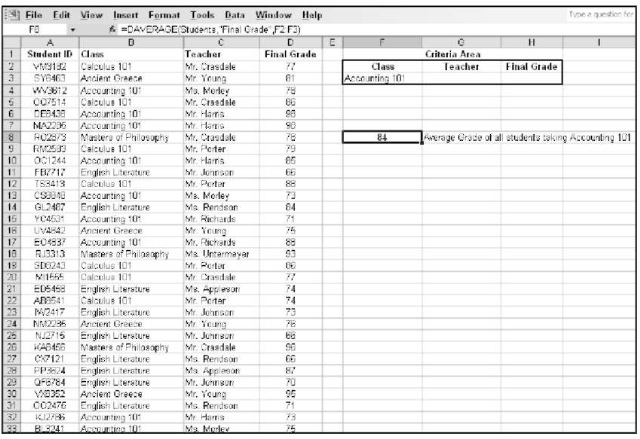
Figure 17-3:
Selecting criteria to use with a database function.
You may notice that the DAVERAGE formula in Figure 17-3 does not make use of a named criteria area. It usually makes sense to name the database area itself, because this information is usually static. Even if rows are added or deleted, the name updates to reflect the correct range.
Using a named area for the criteria is not so simple. Figure 17-4 shows the Student database with four different criteria areas. These areas have all been named as Criteria!, Criteria2, Criteria3, and Criteria4. (How’s that for original?)
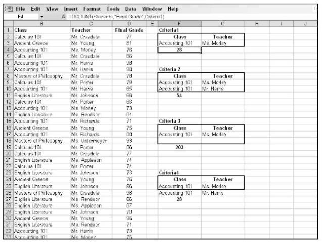
Figure 17-4:
Using named criteria areas.
Each criteria area has a thick border around it. The name is above each one, and a calculated value is below each one. Although all four calculations are trying to calculate similar answers, only the first and second are correct.
| Cell | Formula | |
| F4 | =DCOUNT(Students,”Final | Grade”,Criteria1) |
| F11 | =DCOUNT(Students,”Final | Grade”,Criteria2) |
| F19 | =DCOUNT(Students,”Final | Grade”,Criteria3) |
| F27 | =DCOUNT(Students,”Final | Grade”,Criteria4) |
The problem isn’t the formulas; instead, the problem is the result of how the named criteria areas are used. Essentially, the named areas are prone to providing too much or not enough criteria. Table 17-1 summarizes how the named criteria areas are returning correct or incorrect results.
| Table 17-1 | Why Named Criteria Areas Are a Problem | |
| Criteria Area Name | Criteria Range | What Happens |
| Criterial | F2:G3 | The criteria say to use the records where the class is Accounting 101 and the teacher is Ms. Morley. The size of the named criteria matches the criteria itself and the correct answer is calculated. |
| Criteria2 | F8:G10 | The criteria say to use the records where the class is Accounting 101 and the teacher is either Ms. Morley or Mr. Harris. The size of the named criteria matches the criteria itself and the correct answer is calculated. |
| Criteria3 | F16:G18 | The criteria, unintentionally, say to use the records where the class is Accounting 101 and the teacher is Ms. Morley, or where the class and teacher don’t matter. Because the named criteria area is larger than the supplied criterions and contains a couple of blank cells, the function returns a result based on incorrect criteria. The result is that all the database records are used in the calculation. |
| Criteria4 | F24:G25 | The intention is for the criteria to say to use the records where the class is Accounting 101 and the teacher is either Ms. Morley or Mr. Harris. However the named criteria area is too small and, therefore, the calculation does not take Mr. Harris into account. |
Giving the criteria area a name may not make sense. If the amount of criteria used changes from time to time, then using a fixed area may give incorrect results. In this case, you’re better off just typing in the range address where the criteria are located. If the size of the criteria and the amount of criteria stay constant, then a named area makes sense.
Here’s how you enter any of the database functions. This example uses the DSUM function but the instructions are the same for all the database functions:
1. Import or create a database of information on a worksheet.
The information should be in contiguous rows and columns. Be sure to use field headers.
2. Optionally, use the Define Name dialog box to give the database a name.
To name your database, see the section on “Establishing your database.”
3. Select a portion of the worksheet to be the criteria area, then provide headers in this area that match database headers.
You only have to provide criteria headers for database fields that criteria are applied to. For example, your database area may have 10 columns, but you only apply criteria on 3 columns. Therefore the criteria area can be 3 columns wide.
4. Position the cursor in the cell where you want the results to appear.
This cell must not be in the database area or the criteria area.
5. Enter =DSUM( to begin the function entry.
6. Enter the range of the database, or a name if one is set.
7. Enter a comma (,).
8. Either enter the header name, in quotes, of the database field that the function should process, or just enter the column number.
9. Enter a comma (,).
10. Enter the range of the criteria area.
11. Enter a closing parenthesis to end the function, and press Enter.
Adding Up Only What Matters with DSUM
The DSUM function lets you sum up numbers in a database column for just those rows that match the criteria you specify. Figure 17-5 shows an example using DSUM. The hypothetical students in Accounting 101 decided that the class that scored the highest cumulative grade would throw the end-of-the-school-year party (there are three different teachers). Because the class sizes are close, the students didn’t worry whether any single class would have an advantage. After all, a smaller class filled with bright students can beat a larger class with a few students that get a low grade.
To calculate this, three criteria areas are created. All three set Accounting 101 as the class, but then each criteria area uses a different teacher to filter records. Thus, there are three different answers, in cells F12:F14. Each of the cells holds an identical formula, except for where the DSUM function looks for criteria. For example, here is the formula in cell F14:
![]()
Figure 17-5 shows how the worksheet is set up to calculate this problem. Ms. Morley’s class has the highest overall grade. We hear there will be pizza, ice cream cake, and a stand-up comedian. See you there!
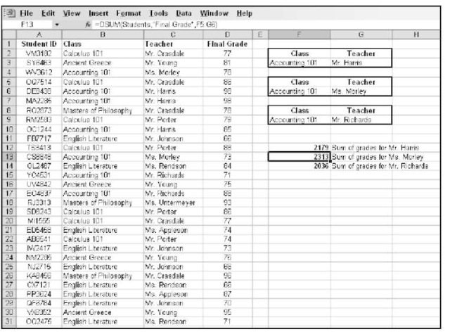
Figure 17-5:
Calculating the sum of grades with the DSUM function.
Going For the Middle with DAVERAGE
The DAVERAGE function lets you find an average for a group of numbers in a database column, for just the rows that match the criteria.
Figure 17-6 shows a worksheet in which the average grade for each course has been calculated. For example, cell G22 shows the average grade for English Literature. Here is the formula:
![]()
Each calculated average uses a different criteria area. Each area filters the result by a particular course. In all cases, the criteria area for the Teacher is left blank. Therefore, the results are based on all students taking the course, regardless of who teaches the course.
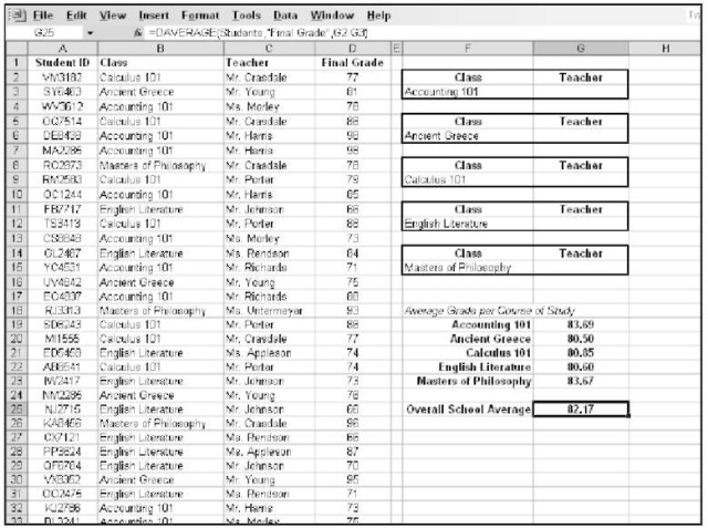
Figure 17-6:
Calculating the average grade per course of study.
For the sake of comparison, DAVERAGE is also used in cell G25 to show the overall school average. Because a criterion is a required function argument, the calculation in cell G25 is set to look at an empty cell. None of the Class criteria cells are free, so the function looks to the Teacher criterion in cell G3. Because this cell has no particular teacher entered as a criterion, the entire database is used to create the result. Here is the formula in cell G25:
![]()
It doesn’t matter which field header is used in the criterion when getting a result based on all records in a database. What does matter is that there is no actual criterion underneath the header.
Counting Only What Counts With DCOUNT
The DCOUNT function lets you calculate a count of records, or rows, that match the criteria.
Figure 17-7 shows how DCOUNT is used to count how many students are in each course. Cells G19:G23 contain formulas that count records based on the criterion (the CLASS) in the associated criteria sections. Here is the formula used in cell G21, which counts the number of students in Calculus 101:
![]()
Note that DCOUNT requires a column of numbers to count on. Therefore, the Final Grade heading is put in the function. Using Class or Teacher to count on would result in zero. Having to use a column that specifically has numbers may seem a little odd. The function is not summing the numbers, it just counts the number of records. But what the heck? It works.
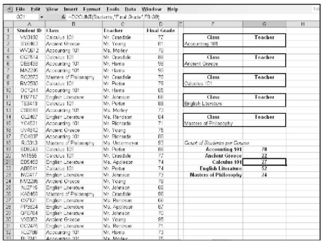
Figure 17-7:
Calculating the number of students per course of study.
Let’s take this a step further. How about counting the number of students who got a grade of 90 or better? How can this be done?
This calculation requires a change in the criterion. You’re no longer looking to segregate answers by Class. So, one criteria section will do, only now you’re filtering on the actual grade. Figure 17-8 shows a worksheet with this type of criterion.
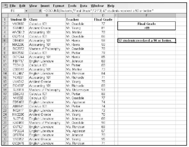
Figure 17-8:
Calculating the number of students that earned a certain grade.
The result in cell F6 concatenates the answer from the DCOUNT function with a string of text. The formula looks like this:

The criterion specifically states to use all records where the Final Grade is greater than 89.
Finding the Highest and Lowest Values
The DMIN and DMAX functions find the minimum or maximum value, respectively, in a database column, for just the rows that match the criteria. Figure 17-9 shows how these two functions have been used to find the highest and lowest grade for English Literature.
The formulas in cells F8 and F10 are practically identical. Here is the formula in cell F8:

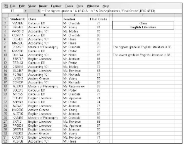
Figure 17-9:
Calculating the highest and lowest grades.
Using DGET to Find Duplicate Values
DGET is a unique database function. It returns three possible values:
If one record matches based on the criteria, DGET returns the criteria.
If no records match based on the criteria, DGET returns the #VALUE! error.
If more than one record matches based on the criteria, DGET returns the
#NUM! error.
By building in a test to see if DGET returns an error, you can discover problems with your data. Imagine this: A teacher alerts you that a student is registered twice for his course. Therefore, in the database there probably are two records that have the same Student ID and Class.
Figure 17-10 shows this on a worksheet. The RM2583 Student ID is being tested for duplicate entry in the Calculus 101 course. If there is more than one record, sure enough, an error will appear.
Cell F5 contains a formula that nests the DGET function inside the ISERROR function, and then all of that is inside the IF function. So, if DGET returns an error, return such a message; otherwise, return a different message. Here is the formula:

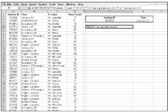
Figure 17-10:
Using DGET to test for duplicate records.
Getting Criteria to Work the Way You Want
Excel’s database functions would not be of much use if you could not create sophisticated queries. A few common query uses include the following:
Find out a result based on criteria that fall between two values (such as a low and high number)
Find out a result based on criteria that have to match all conditions (uses AND logic)
Find out a result based on criteria that have to match any conditions (uses OR logic)
Find out a result based on criteria that match a pattern
Figure 17-11 shows a rather busy worksheet that shows how all these types of queries are assembled. There are several criteria areas and several calculations.
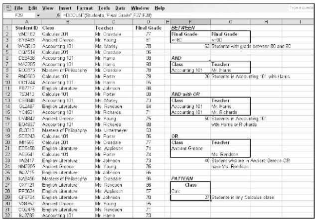
Figure 17-11:
Creating sophisticated queries.
Let’s take each type of query one-by-one. In all these examples, the DCOUNT function is used to count records that meet the criteria.
Finding records that have values in a range
To create criteria that look for records that match a range of values, set up two columns in the criteria area that filter on the same field. Then enter conditions that filter in opposing directions.
Cell F4 reports the count of how many students received a grade between 80 and 90. The criteria used here is in F2:G3. The criteria area has two headers, but they are both for the same field! One of the criterions says to look for records that have a Final Grade of 80 or greater. The other criterion says to look for records that have a Final Grade of 90 or less.
Normally, either one of these criterion conditions would return a greater number when used by itself. For example, if the only criterion was to find records where the Final Grade was 90 or less, then the count would be higher (unless maybe this is M.I.T or Harvard). But taken together, only records that match both of the conditions are counted.
Finding records that must match more than one condition
To create criteria that look for records that must match on more than one field, set up a column in the criteria area for each of the fields. Enter the criteria in the same row.
Cell F9 reports the count of students who are in Accounting 101 and have Mr. Harris for the teacher. The criteria used here is in F7:G8. Both conditions must be met because the criteria conditions are in the same row.
A common query is where one condition is fixed on one value, but the second condition can be based on more than one value. Cell F16 reports the count of students in Accounting 101 that have Mr. Harris or Mr. Roberts. Two conditions must still be met. However, the second criterion can now be more than one value — Mr. Harris or Mr. Roberts. The criteria used here is in F13:G15.
Finding records that match one or more conditions
To create criteria that look for records that can match on one field or another, set up a column in the criteria area for each of the fields. However, do not enter the actual criteria in the same row. Instead, enter the criteria in different rows. The criteria area must be sized to accommodate this.
Cell F23 reports the count of students that are in the Ancient Greece class or have Ms. Rendson. The criteria used here is in F20:G22.
Finding records that match a pattern
By default, the Excel database functions use partial criteria to find records. To demonstrate this, some of the records have been changed from Calculus 101 to Calculus 201. Now there are students in both classes but they are all in Calc, which serves as a pattern to finding records for both Calculus 101 and Calculus 102.
Cell F29 reports the count of students taking one or the other class, because the criteria (in F27:F28) tells the function to use the partial spelling.
