Non-Linear Filtering of Images (Image Processing) Part 2

Non-Linear Filtering of Images in MATLAB

As its name suggests, the Image Processing Toolbox function medfilt2 performs two-dimensional median filtering (the medfilt function is also available for median filtering of one-dimensional signals). The arguments for medfilt2 are straightforward: the input image, the size of the mask, and an optional third argument specifying how to handle boundary pixels15. The command used to create Figure 4-16c is

The Image Processing Toolbox also contains a very useful function, imnoise, that corrupts an image with various types of noise. This function proves very convenient when performing experiments to determine how effective a fdter is in reducing the effects of noise. The imnoise function knows about the following types of noise:

• Gaussian white noise (also white noise whose magnitude tracks the local variance of the image)

• Poisson noise

• Shot noise

• Speckle noise

For each type, imnoise accepts parameters to adjust the characteristics of the noise16. For example in the command used to create Figure 4-16b,

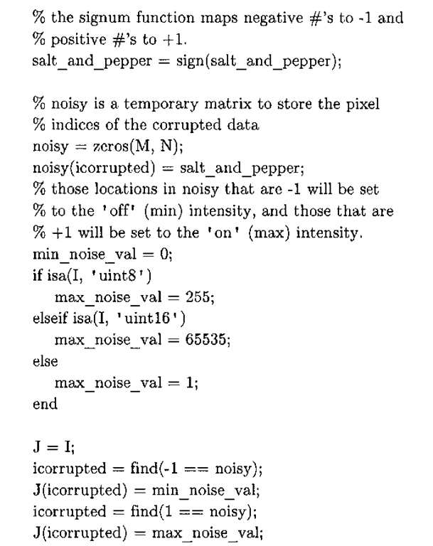
the final argument specifies that the number of corrupted pixels should be 40% of the number of pixels in I. Listing 4-8 is a replacement for the above function that does not require the Image Processing Toolbox, for the single case of salt and pepper (a.k.a. shot) noise.

Listing 4-8: MATLAB function to add salt and pepper noise to an image.

% rand returns a MxN matrix with uniformly distributed

% #’s in the interval (0.0, 1.0), so by finding how

% many of these are less than or equal to how_much, we

% determine which pixels are to be corrupted.

% rand returns a MxN matrix with uniformly distributed

% #’s in the interval (0.0, 1.0), so by finding how

% many of these are less than or equal to how_much, we

% determine which pixels are to be corrupted.

 

% generate a normally distributed vector with zero mean,

% so half of them should be negative, and half of them % positive.

% generate a normally distributed vector with zero mean,

% so half of them should be negative, and half of them % positive.

 

 

 

This function makes extensive use of the built-in MATLAB find function, which accepts a predicate and returns the indices where this predicate evaluates to true. Thus the statement

returns the indices in the matrix R where the value of R is less than or equal to how_much. This begs the question – since R is a 2D matrix, does icorrupted somehow return the row and column numbers for indexing into R? The answer is no, as MATLAB indexes into N-dimensional matrices by assuming a flattened array, akin to how the C programs in this topic index into flattened image buffers. One significant difference between MATLAB and C is that MATLAB is column-major, whereas C is row-major – so while index 2 is the second column in the first row in C, it is the first column in the second row in MATLAB. In MATLAB parlance, the row and column indices are matrix subscripts, and the function ind2sub can then be used to translate between single indices (i.e., the ones returned from find) and subscripts, given the dimensions of a matrix. Similarly, there is a function sub2ind that translates the other way, from multiple subscripts to linear indices.

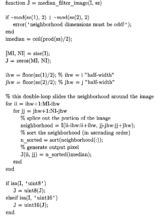
Listing 4-9 is a MATLAB function that may be used as a replacement for medf ilt2, in the event that the Image Processing Toolbox is not available. What is interesting to note about this function’s implementation is how MATLAB’s "colon" notation allows the programmer great flexibility for indexing into images.

Listing 4-9: MATLAB function to perform median filtering of an image.

 

 

 

 

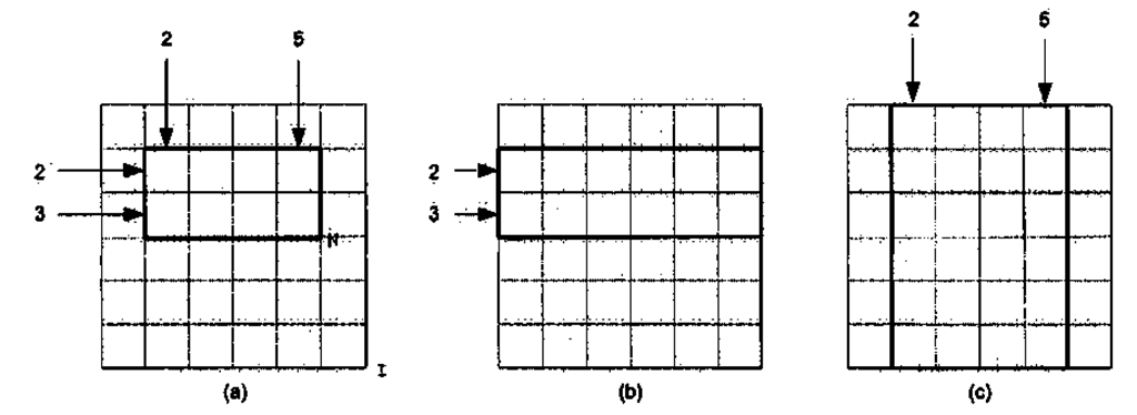
Figure 4-18. MATLAB’s colon notation with 2D matrices, (a) N = 1(2:3, 2 : 5) (b) N = 1(2:3, : ) (c)N = I (:, 2:5)

Given a 2D matrix I, the statement

returns in N the submatrix of I consisting of rows sr (start row) to er (end row) and columns sc (start column) to ec (end column). This notation is used in median_filter_image to extract the sliding window neighborhood at each iteration within the double loop. If either of the two ranges are replaced with just the colon operator, as in I (sr :er, : ) or I (: , sc:ec) then the statement evaluates to every row or column. Figure 4-18 illustrates this situation for the three aforementioned usages of the colon operator.

MATLAB’s colon notation is indicative of the language’s vectorized nature; in well-written MATLAB code, the amount of looping is always kept to a bare minimum. Another usage of the colon operator is to flatten a multidimensional array, as in the statement

Here, neighborhood (:) serves to flatten the 2D neighborhood into a ID array, so that we sort a single vector consisting of all the pixels in the current neighborhood. Without this operation, sort would return n sorted vectors, where n is the number of columns in the median filter mask.

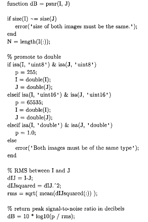
It was stated earlier that with various definitions of the peak signal-to-noise ratio floating around, without an exact definition of what is being quoted this particular metric should be taken with a grain of salt. Perhaps for this very reason, there is not an Image Processing Toolbox function to compare two images numerically, but Listing 4-10 is a simple function psnr that accepts two image matrices of the same type (uint8, uintl6, or double) and returns the PSNR in decibels.

Listing 4-10: MATLAB function that returns the peak signal-to-noise ratio between two images.

The Image Processing Toolbox function nlfilter is an interesting function that can be used to perform generic non-linear filtering of images. This function can be invoked in a few different manners, one of which is

The above statement performs erosion, by passing the image matrix I through a 3×3 minimum filter. The third argument to nlfilter is a string that is treated as a "function pointer", in a similar fashion to bona fide function pointers in C/C++. As the sliding window moves across the image, nlfilter invokes the function referenced by the string using the built-in MATLAB function eval. The function referenced in the call to nlfilter must accept a single input variable x (the current neighborhood) and return a scalar value. In the above case, each neighborhood matrix is first flattened by the colon operator, and the built-in MATLAB min function returns the minimum pixel value for that neighborhood. It is important to understand that this nlfilter call will fail if the colon operator is omitted, i.e. nlfilter (I, [3 3], ‘min (x)’), because min returns a vector of minima from each column if its input is a matrix.

The function pointer string argument to nlfilter is actually shorthand for other forms of invocation. For example the following code snippet implements image dilation:

In the above code, ma x_rep la cement is a sub function passed to nlfilter as a function handle, indicated by the @ symbol. Of course, the function handle can also point to a global MATLAB function, whose implementation is provided in a separate M-file. Function handles are a powerful facility, especially when dealing with classes of algorithms whose basic infrastructure remains the same, but where the individual pixel operations differ. Non-linear filtering of images meets this condition perfectly – a skeleton of the process can be coded in a generic fashion and then the generic function specialized through the use of function handles. In some respects, this design pattern closely follows that of the C++ Standard Template Library (STL), where generic data structures and algorithms are specialized through the use of C++ templates.

A Median Filtering Application Built Using Visual Studio .NET 2003

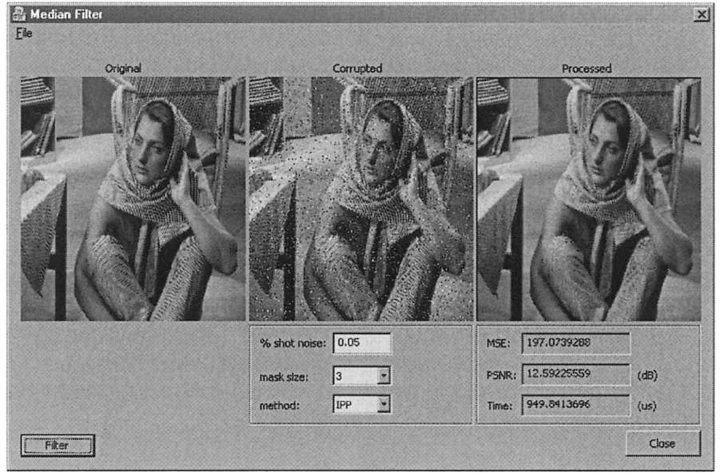
It has been said before but it bears repeating - a working, reference, C/C++ implementation of an algorithm running on the desktop is a major advantage in getting an embedded version of that algorithm running on a DSP. The reasons why are two-fold. Debugging the algorithm in general is substantially easier on the desktop because there are far fewer ancillary issues to deal with (limited memory being one in particular). Moreover, in any real-world system there is more to just getting the image-processing algorithm to work and execute efficiently. The question of whether the particular algorithm works within the application’s context must also be considered. This stage of development can usually be done with simulations using test data, and MATLAB or other equivalent IDEs are a perfect tool for this type of software. Microsoft’s tools are so good, and so amenable to rapid development, that Visual Studio can sometimes be used in lieu of MATLAB, and then you get the added benefit of having a reference implementation to compare against when porting the code over to the DSP. In this section we discuss a median filtering C++ application (located in Chap4\median_filter\MedianFilterVS), that reuses several of the classes first introduced in 3.3.2. A screen-shot of this application is shown in Figure 4.19.

The user loads in a BMP image from the File|Load menu item, adds a parameterized amount of shot noise to the image, and cleans up the image by passing the noisy image through a median filter of size 3×3, 5×5, 7×7, or 1 lxl 1. The efficacy of the processing may be garnered of course through visual inspection of the right-most image display, and MSE and PSNR metrics are computed and displayed. Border pixels are handled in a similar fashion to the linear filtering programs of 4.3 and 4.4 – they are set to zero. Thus, the MSE and PSNR measurements are computed only for the interior portion of the image where pixel values actually change. So for example, with a 3×3 median filter, a subset of the original and processed images are utilized, where the first and last rows and columns are not considered for purposes of comparing the two images.

Just as coding techniques play an important role in DSP optimization, so do they in the desktop realm. To that end, this particular application implements the median filter using five different methods, each of which shall be explained in further detail. The implementation method is selected by using the bottom-most dropdown list box control, and the time taken to filter the image is displayed on the application window, in microseconds.

Figure 4-19. Visual Studio .NET C++ median filtering application.