INTRODUCTION
A major step for high-quality optical devices faults diagnosis concerns scratches and digs defects detection and characterization in products. These kinds of aesthetic flaws, shaped during different manufacturing steps, could provoke harmful effects on optical devices’ functional specificities, as well as on their optical performances by generating undesirable scatter light, which could seriously damage the expected optical features. A reliable diagnosis of these defects becomes therefore a crucial task to ensure products’ nominal specification. Moreover, such diagnosis is strongly motivated by manufacturing process correction requirements in order to guarantee mass production quality with the aim of maintaining acceptable production yield.
Unfortunately, detecting and measuring such defects is still a challenging problem in production conditions and the few available automatic control solutions remain ineffective. That’s why, in most of cases, the diagnosis is performed on the basis of a human expert based visual inspection of the whole production. However, this conventionally used solution suffers from several acute restrictions related to human operator’s intrinsic limitations (reduced sensitivity for very small defects, detection exhaustiveness alteration due to attentiveness shrinkage, operator’s tiredness and weariness due to repetitive nature of fault detection and fault diagnosis tasks).
To construct an effective automatic diagnosis system, we propose an approach based on four main operations: defect detection, data extraction, dimensionality reduction and neural classification. The first operation is based on Nomarski microscopy issued imaging. These issued images contain several items which have to be detected and then classified in order to discriminate between “false” defects (correctable defects) and “abiding” (permanent) ones. Indeed, because of industrial environment, a number of correctable defects (like dusts or cleaning marks) are usually present beside the potential “abiding” defects. Relevant features extraction is a key issue to ensure accuracy of neural classification system; first because raw data (images) cannot be exploited and, moreover, because dealing with high dimensional data could affect learning performances of neural network. This article presents the automatic diagnosis system, describing the operations of the different phases. An implementation on real industrial optical devices is carried out and an experiment investigates a MLP artificial neural network based items classification.
BACKGROUND
Today, the only solution which exists to detect and classify optical surfaces’ defects is a visual one, carried out by a human expert. The first originality of this work is in the sensor used: Normarski microscopy. Three main advantages distinguishing Nomarski microscopy (known also as “Differential Interference Contrast microscopy” (Bouchareine, 1999) (Chatterjee, 2003)) from other microscopy techniques, have motivated our preference for this imaging technique. The first ofthem is related to the higher sensitivity of this technique comparing to the other classical microscopy techniques (Dark Field, Bright Field) (Flewitt & Wild, 1994). Furthermore, the DIC microscopy is robust regarding lighting non-homogeneity. Finally, this technology provides information relative to depth (3-th dimension) which could be exploited to typify roughness or defect’s depth. This last advantage offers precious additional potentiality to characterize scratches and digs flaws in high-tech optical devices. Therefore, Nomarski microscopy seems to be a suitable technique to detect surface imperfections.
On the other hand, since they have shown many attractive features in complex pattern recognition and classification tasks (Zhang, 2000) (Egmont-Petersen, de Ridder, & Handels, 2002), artificial neural network based techniques are used to solve difficult problems. In our particular case, the problem is related to the classification of small defects on a great observation’s surface. These promising techniques could however encounter difficulties when dealing with high dimensional data. That’s why we are also interested in data dimensionality reducing methods.
DEFECTS’ DETECTION AND CLASSIFICATION
The suggested diagnosis process is described in broad outline in the diagram of Figure 1. Every step is presented, first detection and data extraction phases and then classification phase coupled with dimensionality reduction. In a second part, some investigations on real industrial data are carried out and the obtained results are presented.
Detection and Data Extraction
The aim of defect’s detection stage is to extract defects images from DIC detector issued digital image. The proposed method (Voiry, Houbre,Amarger, & Madani, 2005) includes four phases:
• Pre-processing: DIC issued digital image transformation in order to reduce lighting heterogeneity influence and to enhance the aimed defects’ visibility,
• Adaptive matching: adaptive process to match defects,
• Filtering and segmentation: noise removal and defects’ outlines characterization.
• Defect image extraction: correct defect representation construction.
Finally, the image associated to a given detected gives an isolated (from other items) representation of the defect (e.g. depicts the defect in its immediate environment), like depicted in Figure 2.
But, information contained in such generated images is highly redundant and these images don’t have necessarily the same dimension (typically this dimension can turn out to be hundred times as high). That is why this raw data (images) can not be directly processed and has first to be appropriately encoded, using some transformations. Such ones must naturally be invariant with regard to geometric transformations (translation, rotation and scaling) and robust regarding different perturbations (noise, luminance variation and background variation). Fourier-Mellin transformation is used as it provides invariant descriptors, which are considered to have good coding capacity in classification tasks (Choksuriwong, Laurent, & Emile, 2005) (Derrode, 1999) (Ghorbel, 1994). Finally, the processed features have to be normalized, using the centring-reducing transformation. Providing a set of 13 features using such transform, is a first acceptable compromise between industrial environment real-time processing constraints and defect image representation quality (Voiry, Madani, Amarger, & Houbre, 2006).
Figure 1. Block diagram of the proposed defect diagnosis system
Figure 2. Images of characteristic items: (a) Scratch; (b) dig; (c) dust; (d) cleaning marks
Dimensionality Reduction
To obtain a correct description of defects, we must consider more or less important number of Fourier-Mel-lin invariants. But dealing with high-dimensional data poses problems, known as “curse of dimensionality” (Verleysen, 2001). First, sample number required to reach a predefined level of precision in approximation tasks increases exponentially with dimension. Thus, intuitively, the sample number needed to properly learn problem becomes quickly much too large to be collected by real systems, when dimension of data increases. Moreover surprising phenomena appear when working in high dimension (Demartines, 1994): for example, variance of distances between vectors remains fixed while its average increases with the space dimension, and Gaussian kernel local properties are also lost. These last points explain that behaviour of a number of artificial neural network algorithms could be affected while dealing with high-dimensional data. Fortunately, most real-world problem data are located in a manifold of dimension p (the data intrinsic dimension) much smaller than its raw dimension. Reducing data dimensionality to this smaller value can therefore decrease the problems related to high dimension.
In order to reduce the problem dimensionality, we use Curvilinear Distance Analysis (CDA). This technique is related to Curvilinear Component Analysis (CCA), whose goal is to reproduce the topology of a n-dimension original space in a new p-dimension space (where p<n) without fixing any configuration of the topology (Demartines & Herault, 1993). To do so, a criterion characterizing the differences between original and projected space topologies is processed:
Where d^ (respectively dp) is the Euclidean distance between vectors x. and x . of considered distribution in i j original space (resp. in projected space), and F is a decreasing function which favours local topology with respect to the global topology. This energy function is minimized by stochastic gradient descent (Demartines & Herault, 1995):
Where a : ^ [0;1] and X : ^ are two decreasing functions representing respectively a learning parameter and a neighbourhood factor. CCA provides also a similar method to project, in continuous way, new points in the original space onto the projected space, using the knowledge of already projected vectors.
But, since CCA encounters difficulties with unfolding of very non-linear manifolds, an evolution called CDA has been proposed (Lee, Lendasse, Donckers, & Verleysen, 2000). It involves curvilinear distances (in order to better approximate geodesic distances on the considered manifold) instead of Euclidean ones. Curvilinear distances are processed in two steps way. First is built a graph between vectors by considering k-NN, e, or other neighbourhood, weighted by Euclidean distance between adjacent nodes. Then the curvilinear distance between two vectors is computed as the minimal distance between these vectors in the graph using Dijkstra’s algorithm. Finally the original CCA algorithm is applied using processed curvilinear distances. This algorithm allows dealing with very non-linear manifolds and is much more robust against the choices of a and l functions.
It has been successfully used as a preliminary step before maximum likelihood classification in (Lennon, Mercier, Mouchot, & Hubert-Moy, 2001) and we have also showed its positive impact on neural network technique based classification performance (Voiry, Madani, Amarger, & Bernier, 2007). In this last paper, we have first demonstrated that a synthetic problem (nevertheless defined from our real industrial data) whose intrinsic dimensionality is two, is better treated by MLP after 2D dimension reduction than in its raw expression. We have also showed that CDA performs better for this problem than CCA and Self Organizing Map pre-processing.
Implementation on Industrial Optical Devices
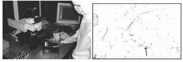
In order to validate the above-presented concepts and to provide an industrial prototype, an automatic control system has been realized. It involves an Olympus B52 microscope combined with a Corvus stage, which allows scanning an entire optical component (presented in Figure 3). 50x magnification is used, that leads to microscopic 1.77 mm x 1.33 mm fields and 1.28 ^m x 1.28 ^m sized pixels. The proposed image processing method is applied on-line. A post-processing software enables to collect pieces of a defect that are detected in different microscopic fields (for example pieces of a long scratch) to form only one defect, and to compute an overall cartography of checked device (Figure 3).
These facilities were used to acquire a great number of Nomarski images, from which were extracted defects images using aforementioned technique. Two experiments called A and B were carried out, using two different optical devices. Table 1 shows the different parameters corresponding to these experiments. It’s important to note that, in order to avoid false classes learning, items images depicting microscopic field boundaries or two (or more) different defects were discarded from used database. Furthermore, studied optical devices were not specially cleaned, what accounts for the presence of some dusts and cleaning marks. Items of these two databases were labelled by an expert with two different labels: “dust” (class1) and “other defects” (class -1). Table 1 shows also items repartition between the two defined classes.
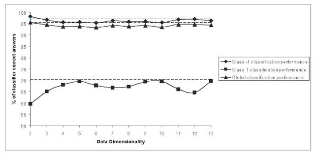
Using this experimental set-up, classification experiment was performed. It involved a multilayer perceptron with n input neurons, 35 neurons in one hidden layer, and 2 output neurons (n-35-2) MLP. First this artificial neural network was trained for discrimination task between classes 1 and -1, using database B. This training phase used BFGS (Broyden, Fletcher, Goldfarb, and Shanno) with Bayesian regularization algorithm, and was achieved 5 times. Subsequently, the generalization ability of obtained neural network was processed using database A. Since database A and B issued from different optical devices, such generalization results are significant. Following this procedure, 14 different experiments were conducted with the aim of studying the global classification performance and the impact of CDA dimensionality reduction on this performance. First experiment used original Fourrier-Mellin issued features (13-dimensional), the others used the same features after CDA n-dimensional space reduction (with n varying between 2 and 13). Figure 4 depicts global classification performances (calculated by averaging percentage of well-classified items for the 5 trainings) for the 14 different experiments, as well as class 1 classification and class -1 classification performances. It shows first that equivalent performances can be obtained using only 5-dimensional data instead of unprocessed defects representations (13-dimensional). As a consequence neural architecture complexity and therefore processing time can be saved using CDA dimensionality reduction, while keeping performance level. Moreover, obtained scores are satisfactory: about 70% of “dust” defects are well-recognized (this can be enough for aimed application) as well as about 97% of other defects (the few 3% errors can however pose problems because every “permanent” defect has to be reported). Furthermore, we think that this significant performances difference between class 1 and class -1 recognition is due to the fact that class 1 is underrep-resented in learning database.
Figure 3. Automatic control system and cartography ofa 100mm x 65mm optical device
Table 1. Description ofthe two databases used for validation experiments
| Database | Optical
Device |
Number of microscopic fields | Corresponding area | Total items number | Class 1 items number | Class -1 items number |
| A | 1 | 1178 | 28 cm2 | 3865 | 275 | 3590 |
| B | 2 | 605 | 14 cm2 | 1910 | 184 | 1726 |
Figure 4. Classification performances for different CDA issued data dimensionality. Classification performances using raw data (13-dimensional) are also depicted as dotted lines.
FUTURE TRENDS
Next phase of this work will deal with classification tasks involving more classes. We want also use much more Fourier-Mellin invariants, because we think that it would improve classification performance by supplying additional information. In this case, CDA based dimensionality reduction technique would be a foremost step to keep reasonable classification system’s complexity and processing time.
CONCLUSION
A reliable diagnosis of aesthetic flaws in high-quality optical devices is a crucial task to ensure products’ nominal specification and to enhance the production quality by studying the impact of the process on such defects. To ensure a reliable diagnosis, an automatic system is needed to detect defects and secondly dis criminate the “false” defects (correctable defects) from “abiding” (permanent) ones. In this paper is described a complete framework, which allows detecting all defects present in a raw Nomarski image and extracting pertinent features for classification of these defects. Obtained proper performances for “dust” versus “other” defects classification task with MLP neural network has demonstrated the pertinence of proposed approach. In addition, data dimensionality reduction permits to use low complexity classifier (while keeping performance level) and therefore to save processing time.
KEY TERMS
Artificial Neural Networks: A network of many simple processors (“units” or “neurons”) that imitates a biological neural network. The units are connected by unidirectional communication channels, which carry numeric data. Neural networks can be trained to find nonlinear relationships in data, and are used in applications such as robotics, speech recognition, signal processing or medical diagnosis.
Backpropagation algorithm: Learning algorithm of ANNs, based on minimising the error obtained from the comparison between the outputs that the network gives after the application of a set of network inputs and the outputs it should give (the desired outputs).
Classification: Affectation of a phenomenon to a predefined class or category by studying its characteristic features. In our work it consists in determining the nature of detected optical devices surface defects (for example “dust” or “other type of defects”).
Data Dimensionality Reduction: Data dimensionality reduction is the transformation of high-dimensional data into a meaningful representation of reduced dimensionality. The goal is to find the important relationships between parameters and reproduce those relationships in a lower dimensionality space. Ideally, the obtained representation has a dimensionality that corresponds to the intrinsic dimensionality of the data. Dimensionality reduction is important in many domains, since it facilitates classification, visualization, and compression of high-dimensional data. In our work it’s performed using Curvilinear Distance Analysis.
Data Intrinsic Dimension: When data is described by vectors (sets of characteristic values), data intrinsic dimension is the effective number of degrees of freedom of the vectors’ set. Generally, this dimension is smaller than the data raw dimension because it may exist linear and/or non-linear relations between the different components of the vectors.
Data Raw Dimension: When data is described by vectors (sets of characteristic values), data raw dimension is simply the number of components of these vectors.
Detection: Identification of a phenomenon among others from a number of characteristic features or “symptoms”. In our work, it consists in identifying surface irregularities on optical devices.
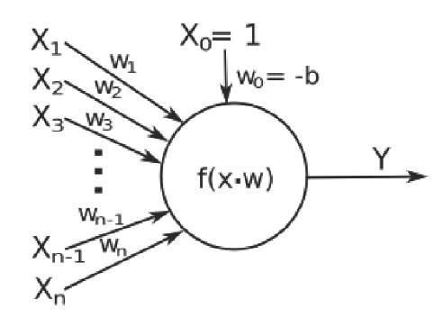
MLP (Multi Layer Perceptron): This widely used artificial neural network employs the perceptron as simple processor. The model of the perceptron, proposed by Rosenblatt is as follows:
In this diagram, the X represent the inputs and Y the output of the neuron. Each input is multiplied by the weight w, a threshold b is subtracted from the result and finally Y is processed by the application of an activation function f. The weights of the connection are ad.usted during a learning phase using backpropa-gation algorithm.


