Overview
In computer graphics, blending curves and surfaces are widely used for both interpolation and approximation. We have previously seen the application of Hermite polynomials in vertex blending, and Catmull-Rom splines for keyframe interpolation. Spline curves and surfaces also find applications in the interactive design of three-dimensional models.
This topic gives an overview of polynomial interpolation methods, and the construction of splines using different types of piecewise cubic polynomial curves. Design aspects such as local control, flexibility and parametric continuity are discussed in detail. Surface design techniques using two-dimensional Bezier and B-spline surface patches are also presented. Extensions of these methods using rational basis functions are then outlined.
Polynomial Interpolation
Suppose we are given n points (x,, y,), i = 1… n, on the xy-plane where all x,s are distinct. The polynomial interpolation theorem states that there is a unique polynomial f (x) of degree n — 1 such that
The above equation shows that the polynomial curve given by y = f (x) passes through all the n points. Such a curve that passes through all input points is called an interpolating curve. On the other hand, a curve that passes through only a few of the input points is called an approximating curve. The Bezier spline (see Box 2.4, Sect. 2.7) is an example of an approximating curve.
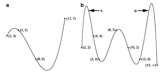
Fig. 7.1 Polynomial interpolation curves of (a) degree 3, and (b) degree 6
Consider the polynomial of degree n — 1 given by
The above function attains a value 1 if x = x1, and 0 if x = x2,…, xn. We can therefore combine such polynomials to form the required interpolating polynomial f (x):
The polynomials c(x) are the Lagrange polynomials of degree n — 1 given by
As an example, four points (3, 4), (5, 5), (8, 0), (13, 7) are used to construct a cubic polynomial curve in Fig. 7.1a. Another interpolating curve through seven points is shown in Fig. 7.1b.
Interpolation curves of degree higher than three can potentially have large overshoots (marked ‘A’ in Fig. 7.1b), or undesirable oscillations (marked ‘B’ in Fig. 7.1b). Such curves, even though they pass through all the user input points, may not describe the shape represented by those points. Piecewise polynomial curves of a low degree are therefore commonly used for approximating shapes.
The system of equations in Eq. 7.1 can also be written as a matrix equation Y = VA :
where the polynomial is assumed to have the form
The coefficients a, of the polynomial can be obtained by taking the matrix inverse: A = V “ 1Y. The n x n matrix V is called the Vandermonde matrix. Since x,s are all distinct, this matrix is invertible.
We now look at a simple and efficient method for evaluating polynomials of the form in Eq. 7.6. If we use the formula xk = x.xk ~ 1 to compute the powers of x for evaluating the terms of the polynomial from left to right, we need to perform 2(n — 1) multiplications and n — 1 additions. The Horner’s method is used to reduce the number of multiplications by rearranging the polynomial as a nested set of expressions:
Each nested sub-expression in the above equation requires one multiplication and one addition. Evaluating the polynomial from the innermost expression requires a total of only n — 1 multiplications.
Cubic Parametric Curves
Cubic polynomials have the advantage that they can be easily evaluated and used to generate small curve segments of an interpolating spline with sufficient flexibility. A cubic polynomial curve can meet four constraints simultaneously such as the requirement to pass through four distinct points, or a requirement to pass through two points and have user specified tangent directions at those points. Splines commonly use parametric representations of piecewise cubic curves defined using three polynomials in a single parameter t:
The above polynomials are called the x-polynomial, y-polynomial and z-polynomial respectively. The parameter t usually varies from 0 to 1, with each value of t corresponding to a single point P(t) = (x(t), y(t), z(t)) on the curve. The polynomials thus define a mapping from an interval in the onedimensional parameter space to a set of points in the three-dimensional space. A common example is where t represents time, and P(t) the position of a moving point at that instant. The equation for x(t) given above can be re-written as follows:
The polynomial coefficients a;, b;, c; are computed using a set of control points and continuity constraints. As an example, consider the requirement that the cubic curve needs to pass through four distinct points P; = (x;, y;, z;), i = 1… 4. If t; denotes the values of the parameter t corresponding to the four control points, we have
This equation is the cubic version of Eq. 7.5. The 4 x 4 Vandermonde matrix is invertible if all t;s are distinct. We write this equation in a concise form as Gx = VA, or equivalently as A = V “ 1Gx, where Gx is a column vector containing only the x-coordinates of the control points. The inverse V “ 1 of the Vandermonde matrix can be computed as the product UL, where U is the following upper triangular matrix
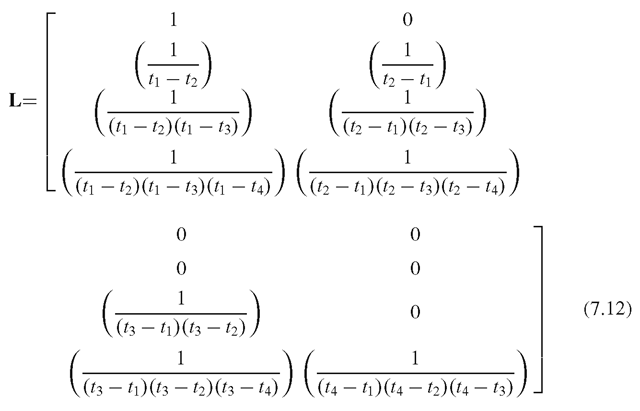
and L is a lower triangular matrix given by
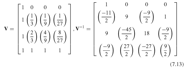
For example, if the parametric values are equally spaced in the interval [0, 1], so that t1 = 0, t2 = 1/3, t3 = 2/3, t4 = 1, then we have the following values for V and V – 1:
From Eq. 7.9, we now have
The product TV – 1 is a row vector containing four functions of the parameter t. Thus the above equation can be rewritten as
Fig. 7.2 Piecewise cubic interpolation polynomials constructed using groups of four points
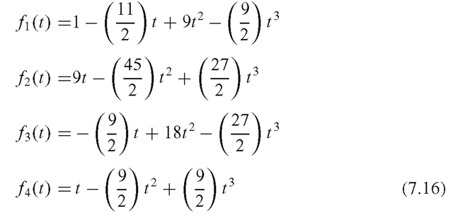
For the example in Eq. 7.13, we have
The functions f (t) are called blending polynomials. Note that the sum of the above functions is 1 for all values of t. Generalising Eq. 7.15, and since the blending polynomials are common for x, y, and z axes, we find that
We can thus write the parametric equation for the cubic curve as a combination of the control points:
Figure 7.2 shows a set of points j oined together using piecewise cubic polynomial curves through groups of four points, constructed using the above equation. Each cubic polynomial curve is called a segment.
The matrix V – 1 is sometimes denoted by M, and referred to as the basis matrix. With this notation, the blending functions and the basis matrix are related as follows:
The points where the polynomial curves meet are called knots. It is often desirable to have tangential and higher order continuity at the knots. Such curves are called splines. In the next section, we discuss different orders of continuity constraints that can be used in the design of interpolating curves and surfaces.


