Analysis of dispersion:
Synonym for multivariate analysis of variance.
Analysis of variance (ANOVA):
The separation of variance attributable to one cause from the variance attributable to others. By partitioning the total variance of a set of observations into parts due to particular factors, for example, sex, treatment group etc., and comparing variances (mean squares) by way of F-tests, differences between means can be assessed. The simplest analysis of this type involves a one-way design, in which N subjects are allocated, usually at random, to the k different levels of a single factor. The total variation in the observations is then divided into a part due to differences between level means (the between groups sum of squares) and a part due to the differences between subjects in the same group (the within groups sum of squares, also known as the residual sum of squares). These terms are usually arranged as an analysis of variance table.
| Source | df | SS | MS | MSR | ||
| Bet. grps. | k – 1 | SSB | SSB/(k - | 1) | ssb/(k-ssw/(N- | -1) -k) |
| With. grps. | N – k | SSW | SSW/(N | - k) | ||
| Total | N – 1 |
SS = sum of squares; MS = mean square; MSR = mean square ratio.
If the means of the populations represented by the factor levels are the same, then within the limits of random variation, the between groups mean square and within groups mean square, should be the same. Whether this is so can, if certain assumptions are met, be assessed by a suitable F-test on the mean square ratio. The necessary assumptions for the validity of the F-test are that the response variable is normally distributed in each population and that the populations have the same variance. Essentially an example of the generalized linear model with an identity link function and normally distributed error terms. See also analysis of covariance, parallel groups design and factorial designs.
Analytic epidemiology:
A term for epidemiological studies, such as case-controlstudies, that obtain individual-level information on the association between disease status and exposures of interest.
Ancillary statistic:
A term applied to the statistic C in situations where the minimal sufficient statistic, S, for a parameter 0, can be written as S = (T, C) and C has a marginal distribution not depending on 0. For example, let N be a random variable with a known distribution pn = Pr(N = n)(n = 1, 2,…), and let Y1, Y2,…, YN be independently and identically distributed random variables from the exponential family distribution with parameter, 0. The likelihood of the data (n, y1, y2,…, yn) is
so that S = Ej=1 b(Yj), N] is sufficient for 0 and N is an ancillary statistic. Important in the application of conditional likelihood for estimation.
ANCOVA:
Acronym for analysis of covariance.
Anderson-Darling test:
A test that a given sample of observations arises from some specified theoretical probability distribution. For testing the normality of the data, for example, the test statistic is
where x^ < xp) <• • • < X(n) are the ordered observations, s2 is the sample variance, and
where
The null hypothesis of normality is rejected for ‘large’ values of A. Critical values of the test statistic are available. See also Shapiro-Wilk test.
Anderson-Gill model:
A model for analysing multiple time response data in which each subject is treated as a multi-event counting process with essentially independent increments.
Anderson, John Anthony (1939-1983):
Anderson studied mathematics at Oxford, obtaining a first degree in 1963, and in 1968 he was awarded a D.Phil. for work on statistical methods in medical diagnosis. After working in the Department of Biomathematics in Oxford for some years, Anderson eventually moved to Newcastle University, becoming professor in 1982. Contributed to multivariate analysis, particularly discriminant analysis based on logistic regression. He died on 7 February 1983, in Newcastle.
Anderson, Oskar Nikolayevick (1887-1960):
Born in Minsk, Byelorussia, Anderson studied mathematics at the University of Kazan. Later he took a law degree in St Petersburg and travelled to Turkestan to make a survey of agricultural production under irrigation in the Syr Darya River area. Anderson trained in statistics at the Commercial Institute in Kiev and from the mid-1920s he was a member of the Supreme Statistical Council of the Bulgarian government during which time he successfully advocated the use of sampling techniques. In 1942 Anderson accepted an appointment at the University of Kiel, Germany and from 1947 until his death he was Professor of Statistics in the Economics Department at the University of Munich. Anderson was a pioneer of applied sample-survey techniques.
Andrews’ plots:
A graphical display of multivariate data in which an observation, x’ = [x1, x2,..., xq] is represented by a function of the form
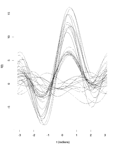
plotted over the range of values — n < t < n. A set of multivariate observations is displayed as a collection of these plots and it can be shown that those functions that remain close together for all values of t correspond to observations that are close to one another in terms of their Euclidean distance. This property means that such plots can often be used to both detect groups of similar observations and identify outliers in multivariate data. The example shown at Fig. 3 consists of plots for a sample of 30 observations each having five variable values. The plot indicates the presence of three groups in the data. Such plots can cope only with a moderate number of observations before becoming very difficult to unravel.
Fig. 3 Andrews’ plot for 30, five-dimensional observations constructed to contain three relatively distinct groups.
Angle count method:
A method for estimating the proportion of the area of a forest that is actually covered by the bases of trees. An observer goes to each of a number of points in the forest, chosen either randomly or systematically, and counts the number of trees that subtend, at that point, an angle greater than or equal to some predetermined fixed angle 2a. [Spatial Data Analysis by Example, Volume 1, 1985, G. Upton and B. Fingleton, Wiley, New York.]
Angler survey:
A survey used by sport fishery managers to estimate the total catch, fishing effort and catch rate for a given body of water. For example, the total effort might be estimated in angler-hours and the catch rate in fish per angler-hour. The total catch is then estimated as the product of the estimates of total effort and average catch rate. [Fisheries Techniques, 1983, L.A. Nielson and D.C. Johnson, eds., American Fisheries Society, Bethesda, Maryland.]
Angular histogram:
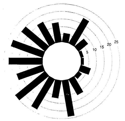
A method for displaying circular data, which involves wrapping the usual histogram around a circle. Each bar in the histogram is centred at the midpoint of the group interval with the length of the bar proportional to the frequency in the group. Figure 4 shows such a display for arrival times on a 24 hour clock of 254 patients at an intensive care unit, over a period of 12 months.
Fig. 4 Angular histogram for arrival times at an intensive care unit.
Angular transformation:
Synonym for arc sine transformation.
Angular uniform distribution:
A probability distribution for a circular random variable, 0, given by
Annealing algorithm:
Synonym for simulated annealing.
ANOVA:
Acronym for analysis of variance.
Ansari-Bradley test:
A test for the equality of variances of two populations having the same median. The test has rather poor efficiency relative to the F-test when the populations are normal. See also Conover test and Klotz test.
Anscombe residual:
A residual based on the difference between some function of the observed value of a response and the same function of the fitted value under some assumed model. The function is chosen to make the residuals as normal as possible and for generalized linear models is obtained from
where V(x) is the function specifying the relationship between the mean and variance of the response variable of interest. For a variable with a Poisson distribution, for 2 ^2 example, V(x) = x and so residuals might be based on y3 — y3.
Antidependence models:
A family of structures for the variance-covariance matrix of a set of longitudinal data, with the model of order r requiring that the sequence of random variables, Y1y Y2,…, YT is such that for every t > r
is conditionally independent of Yt—r—j,…, Yj. In other words once account has been taken of the r observations preceding Yt, the remaining preceding observations carry no additional information about Yt. The model imposes no constraints on the constancy of variance or covariance with respect to time so that in terms of second-order moments, it is not stationary. This is a very useful property in practice since the data from many longitudinal studies often have increasing variance with time.
Anthropometry:
A term used for studies involving measuring the human body. Direct measures such as height and weight or indirect measures such as surface area may be of interest. See also body mass index.
Anti-ranks:
For a random sample X1,…, Xn, the random variables D1,…, Dn such that
If, for example, D1 = 2 then X2 is the smallest absolute value and Z1 has rank 1.
Antithetic variable:
A term that arises in some approaches to simulation in which successive simulation runs are undertaken to obtain identically distributed unbiased run estimators that rather than being independent are negatively correlated. The value of this approach is that it results in an unbiased estimator (the average of the estimates from all runs) that has a smaller variance than would the average of identically distributed run estimates that are independent. For example, if r is a random variable between 0 and 1 then so is s = 1 — r. Here the two simulation runs would involve r1, r2, …, rm and 1 — r1, 1 — r2, …, 1 — rm, which are clearly not independent.
A posteriori comparisons:
Synonym for post-hoc comparisons.
Apparent error rate:
Synonym for resubstitution error rate.
Approximate bootstrap confidence (ABC) method:
A method for approximating confidence intervals obtained by using the bootstrap approach, that do not use any Monte Carlo replications.
Approximation:
A result that is not exact but is sufficiently close for required purposes to be of practical use.
A priori comparisons:
Synonym for planned comparisons.
Aranda-Ordaz transformations:
A family of transformations for a proportion, p, given by
When a = 1, the formula reduces to the logistic transformation of p. As a ! 0 the result is the complementary log-log transformation.
Arbuthnot, John (1667-1735):
Born in Inverbervie, Grampian, Arbuthnot was physician to Queen Anne from 1709 until her death in 1714. A friend of Jonathan Swift who is best known to posterity as the author of satirical pamphlets against the Duke of Marlborough and creator of the prototypical Englishman, John Bull. His statistical claim to fame is based on a short note published in the Philosophical Transactions of the Royal Society in 1710, entitled ‘An argument for Divine Providence, taken from the constant regularity observ’d in the births of both sexes.’ In this note he claimed to demonstrate that divine providence, not chance governed the sex ratio at birth, and presented data on christenings in London for the eighty-two-year period 1629-1710 to support his claim. Part of his reasoning is recognizable as what would now be known as a sign test. Arbuthnot was elected a Fellow of the Royal Society in 1704. He died on 27 February 1735 in London.
Archetypal analysis:
An approach to the analysis of multivariate data which seeks to represent each individual in the data as a mixture of individuals of pure type or archetypes. The archetypes themselves are restricted to being mixtures of individuals in the data set. Explicitly the problem is to find a set of q x 1 vectors z1,…, zp that characterize the archetypal patterns in the multivariate data, X. For fixed z1,…, zp where
under the constraints, aik > 0, J2aik = 1. Then define the archetypal patterns or archetypes as the mixtures z1,…, zp that minimize
For p > 1 the archetypes fall on the convex hull of the data; they are extreme data values such that all the data can be represented as convex mixtures of the archetypes. However, the archetypes themselves are not wholly mythological because each is constrained to be a mixture of points in the data. [Technometrics, 1994, 36, 338-47.]
Arc sine distribution:
A beta distribution with a = p = 0.5.
Arc sine law:
An approximation applicable to a simple random walk taking values 1 and — 1 with probabilities 1 which allows easy computation of the probability of the fraction of time that the accumulated score is either positive or negative. The approximation can be stated thus; for fixed a (0 < a < 1) and n the probability that the fraction k/n of time that the accumulated score is positive is less than a tends to
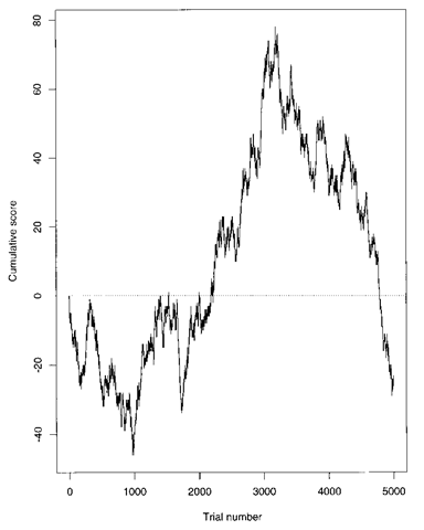
For example, if an unbiased coin is tossed once per second for a total of 365 days, there is a probability of 0.05 that the more fortunate player will be in the lead for more than 364 days and 10 hours. Few people will believe that a perfect coin will produce sequences in which no change of lead occurs for millions of trials in succession and yet this is what such a coin will do rather regularly. Intuitively most people feel that values of k/n close to 1 are most likely. The opposite is in fact true. The possible values close to 2 are least probable and the extreme values k/n = 1 and k/n = 0 are most probable. Figure 5 shows the results of an experiment simulating 5000 tosses of a fair coin (Pr(Heads) = Pr(Tails) = 2) in which a head is given a score of 1 and a tail —1. Note the length of the waves between successive crossings of y = 0, i.e., successive changes of lead.
Fig. 5 Result of 5000 tosses of a fair coin scoring 1 for heads and —1 for tails.
Arc sine transformation:
A transformation for a proportion, p, designed to stabilize its variance and produce values more suitable for techniques such as analysis of variance and regression analysis. The transformation is given by
ARE:
Abbreviation for asymptotic relative efficiency.
Area sampling:
A method of sampling where a geographical region is subdivided into smaller areas (counties, villages, city blocks, etc.), some of which are selected at random, and the chosen areas are then subsampled or completely surveyed. See also cluster sampling.
Area under curve (AUC):
Often a useful way of summarizing the information from a series of measurements made on an individual over time, for example, those collected in a longitudinal study or for a dose-response curve. Usually calculated by adding the areas under the curve between each pair of consecutive observations, using, for example, the trapezium rule. Often a predictor of biological effects such as toxicity or efficacy. See also Cmax, response feature analysis and Tmax.
Arfwedson distribution:
The probability distribution of the number of zero values (M0) among k random variables having a multinomial distribution with p1 = p2 = • • • = pk. If the sum of the k random variables is n then the distribution is given by
ARIMA:
Abbreviation for autoregressive integrated moving-average model.
Arjas plot:
A procedure for checking the fit of Cox’s proportional hazards model by comparing the observed and expected number of events, as a function of time, for various subgroups of covariate values.
ARMA:
Abbreviation for autoregressive moving-average model.
Armitage-Doll model:
A model of carcinogenesis in which the central idea is that the important variable determining the change in risk is not age, but time. The model proposes that cancer of a particular tissue develops according to the following process:
• a normal cell develops into a cancer cell by means of a small number of transitions through a series of intermediate steps;
• initially, the number of normal cells at risk is very large, and for each cell a transition is a rare event;
• the transitions are independent of one another.
Armitage-Hill test:
A test for carry-over effect in a two-by-two crossover design where the response is a binary variable.
Artificial intelligence:
A discipline that attempts to understand intelligent behaviour in the broadest sense, by getting computers to reproduce it, and to produce machines that behave intelligently, no matter what their underlying mechanism. (Intelligent behaviour is taken to include reasoning, thinking and learning.) See also artificial neural network hand pattern recognition.
Artificial neural network:
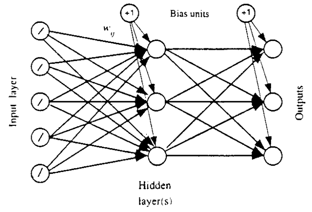
A mathematical structure modelled on the human neural network and designed to attack many statistical problems, particularly in the areas of pattern recognition, multivariate analysis, learning and memory. The essential feature of such a structure is a network of simple processing elements (artificial neurons) coupled together (either in the hardware or software), so that they can cooperate. From a set of ‘inputs’ and an associated set of parameters, the artificial neurons produce an ‘output’ that provides a possible solution to the problem under investigation. In many neural networks the relationship between the input received by a neuron and its output is determined by a generalized linear model. The most common form is the feed-forward network which is essentially an extension of the idea of the perceptron. In such a network the vertices can be numbered so that all connections go from a vertex to one with a higher number; the vertices are arranged in layers, with connections only to higher layers. This is illustrated in Fig. 6. Each neuron sums its inputs to form a total input Xj and applies a function f to Xj to give output y. The links have weights Wj which multiply the signals travelling along them by that factor. Many ideas and activities familiar to statisticians can be expressed in a neural-network notation, including regression analysis, generalized additive models, and discriminant analysis. In any practical problem the statistical equivalent of specifying the architecture of a suitable network is specifying a suitable model, and training the network to perform well with reference to a training set is equivalent to estimating the parameters of the model given a set of data.
Fig. 6 A diagram illustrating a feed-forward network.
Ascertainment bias:
A possible form of bias, particularly in retrospective studies, that arises from a relationship between the exposure to a risk factor and the probability of detecting an event of interest. In a study comparing women with cervical cancer and a control group, for example, an excess of oral contraceptive use among the cases might possibly be due to more frequent screening for the disease among women known to be taking the pill. [SMR Chapter 5.]
ASN:
Abbreviation for average sample number.
As-randomized analysis:
Synonym for intention-to-treat analysis.
Assignment method:
Synonym for discriminant analysis.
Association:
A general term used to describe the relationship between two variables.
Essentially synonymous with correlation. Most often applied in the context of binary variables forming a two-by-two contingency table. See also phi-coefficient and Goodman-Kruskal measures of association.
Assortative mating:
A form of non-random mating where the probability of mating between two individuals is influenced by their phenotypes (phenotypic assortment), genotypes (genotypic assortment) or environments (cultural assortment).
Assumptions:
The conditions under which statistical techniques give valid results. For example, analysis of variance generally assumes normality, homogeneity of variance and independence of the observations.
Asymmetrical distribution:
A probability distribution or frequency distribution which is not symmetrical about some central value. Examples include the exponential distribution and J-shaped distribution.
Asymmetric maximum likelihood (AML):
A variant of maximum likelihood estimation that is useful for estimating and describing overdispersion in a generalized linear model.
Asymmetric proximity matrices:
Proximity matrices in which the off-diagonal elements, in the ith row and jth column and the jth row and ith column, are not necessarily equal. Examples are provided by the number of marriages between men of one nationality and women of another, immigration/emigration statistics and the number of citations of one journal by another. Multidimensional scaling methods for such matrices generally rely on their canonical decomposition into the sum of a symmetric matrix and a skew symmetric matrix.
Asymptotically unbiased estimator:
An estimator of a parameter which tends to being unbiased as the sample size, n, increases. For example,
is not an unbiased estimator of the population variance a2 since its expected value is
but it is asymptotically unbiased. [Normal Approximation and Asymptotic Expansions, 1976, R.N. Bhattacharya and R. Rao, Wiley, New York.]
Asymptotic distribution:
The limiting probability distribution of a random variable calculated in some way from n other random variables, as n ! 1. For example, the mean of n random variables from a uniform distribution has a normal distribution for large n.
Asymptotic efficiency:
A term applied when the estimate of a parameter has a normal distribution around the true value as mean and with a variance achieving the Cramer-Rao lower bound. See also superefficient.
Asymptotic method:
Synonym for large sample method.
Asymptotic relative efficiency:
The relative efficiency of two estimators of a parameter in the limit as the sample size increases.
Atlas mapping:
A biogeographical method used to investigate species-specific distributional status, in which observations are recorded in a grid of cells. Such maps are examples of geographical information systems.
Attack rate:
A term often used for the incidence of a disease or condition in a particular group, or during a limited period of time, or under special circumstances such as an epidemic. A specific example would be one involving outbreaks of food poisoning, where the attack rates would be calculated for those people who have eaten a particular item and for those who have not.
Attenuation:
A term applied to the correlation between two variables when both are subject to measurement error, to indicate that the value of the correlation between the ‘true values’ is likely to be underestimated. See also regression dilution.
Attitude scaling:
The process of estimating the positions of individuals on scales purporting to measure attitudes, for example a liberal-conservative scale, or a risk-willingness scale. Scaling is achieved by developing or selecting a number of stimuli, or items which measure varying levels of the attitude being studied. See also Likert scale and multidimensional scaling.
Attributable response function:
A function N(x, x0) which can be used to summarize the effect of a numerical covariate x on a binary response probability. Assuming that in a finite population there are m(x) individuals with covariate level x who respond with probability n(x), then N(x, x0) is defined as N(x, x0) = m(x){n(x) — n(x0)} The function represents the response attributable to the covariate having value x rather than x0. When plotted against x > x0 this function summarizes the importance of different covariate values in the total response. [Biometrika, 1996, 83, 563-73.]
Attributable risk:
A measure of the association between exposure to a particular factor and the risk of a particular outcome, calculated as
Attributable risk:
A measure of the association between exposure to a particular factor and the risk of a particular outcome, calculated as
Measures the amount of the incidence that can be attributed to one particular factor.
Attrition:
A term used to describe the loss of subjects over the period of a longitudinal study.
May occur for a variety of reasons, for example, subjects moving out of the area, subjects dropping out because they feel the treatment is producing adverse side effects, etc. Such a phenomenon may cause problems in the analysis of data from such studies. See also missing values and Diggle-Kenward model for dropouts.
AUC:
Abbreviation for area under curve.
Audit in clinical trials:
The process of ensuring that data collected in complex clinical trials are of high quality.
Audit trail:
A computer program that keeps a record of changes made to a database.
Autocorrelation:
The internal correlation of the observations in a time series, usually expressed as a function of the time lag between observations. Also used for the correlations between points different distances apart in a set of spatial data (spatial autocorrelation). The autocorrelation at lag k, y(k), is defined mathematically as
where Xt, t = 0, ±1, ±2,… represent the values of the series and is the mean of the series. E denotes expected value. The corresponding sample statistic is calculated as
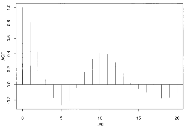
where x is the mean of the series of observed values, x1, x2,…, xn. A plot of the sample values of the autocorrelation against the lag is known as the autocorrelation function or correlogram and is a basic tool in the analysis of time series particularly for indicating possibly suitable models for the series. An example is shown in Fig. 7. The term in the numerator of y(k) is the autocovariance. A plot of the autocovar-iance against lag is called the autocovariance function.
Automatic interaction detector (AID):
A method that uses a set of categorical explanatory variables to divide data into groups that are relatively homogeneous with respect to the value of some continuous response variable of interest. At each stage, the division of a group into two parts is defined by one of the explanatory variables, a subset of its categories defining one of the parts and the remaining categories the other part. Of the possible splits, the one chosen is that which maximizes the between groups sum of squares of the response variable. The groups eventually formed may often be useful in predicting the value of the response variable for some future observation. See also classification and regression tree technique and chi-squared automated interaction detector.
Fig. 7 An example of an autocorrelation function.
Autoregressive model:
A model used primarily in the analysis of time series in which the observation, xt, at time t, is postulated to be a linear function of previous values of the series. So, for example, a first-order autoregressive model is of the form
where at is a random disturbance and 0 is a parameter of the model. The corresponding model of order p is
Xt = 01 Xt-1 + 02 Xt-2 + ••• + 0pXt-p + at
Autoregressive moving-average model: A model for a time series that combines both an autoregressive model and a moving-average model. The general model of order p, q (usually denoted ARMA(p, q)) is
are a white noise sequence. In some cases such models are applied to the time series observations after differencing to achieve stationarity, in which case they are known as autoregressive integrated moving-average models.
Auxiliary variable techniques:
Techniques for improving the performance of Gibbs sampling in the context of Bayesian inference for hierarchical models.
Available case analysis:
An approach to handling missing values in a set of multivariate data, in which means, variances, covariances, etc., are calculated from all available subjects with non-missing values for the variable or pair of variables involved. Although this approach makes use of as much of the data as possible it has disadvantages. One is that summary statistics will be based on different numbers of observations. More problematic however is that this method can lead to variance-covariance matrices and correlation matrices with properties that make them unsuitable for many methods of multivariate analysis such as principal components analysis and factor analysis.
Average:
Most often used for the arithmetic mean of a sample of observations, but can also be used for other measures of location such as the median.
Average age at death:
A flawed statistic summarizing life expectancy and other aspects of mortality. For example, a study comparing average age at death for male symphony orchestra conductors and for the entire US male population showed that, on average, the conductors lived about four years longer. The difference is, however, illusory, because as age at entry was birth, those in the US male population who died in infancy and childhood were included in the calculation of the average life span, whereas only men who survived to become conductors could enter the conductor cohort. The apparent difference in longevity disappeared after accounting for infant and perinatal mortality. [Methodological Errors in Medical Research, 1990, B. Andersen, Blackwell Scientific, Oxford.]
Average deviation:
A little-used measure of the spread of a sample of observations. It is defined as
where x, x2,…, xn represent the sample values, and x their mean.
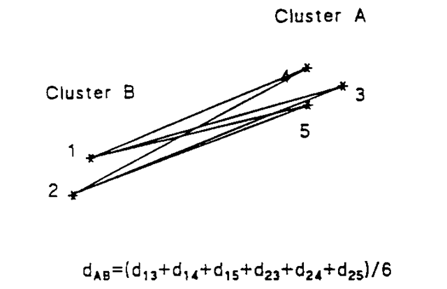
Average linkage: An agglomerative hierarchical clustering method that uses the average distance from members of one cluster to members of another cluster as the measure of inter-group distance. This distance is illustrated in Fig. 8.
Average sample number (ASN)
A quantity used to describe the performance of a sequential analysis given by the expected value of the sample size required to reach a decision to accept the null hypothesis or the alternative hypothesis and therefore to discontinue sampling. [KA2 Chapter 24.]
Fig. 8 Average linkage distance for two clusters.


