Volume Visualization (Plotting in Three Dimensions) (MATLAB) Part 2

Stream Plots

Since vector volume data can be thought of as particles flowing through a volume, it is desirable to have some visualization methods that indicate the direction of flow. Stream plots do just that. The differences amongst the stream plots provided in MATLAB have to do with the way the streams are visualized. Stream plots are typically combined with other visualization techniques, such as slices, in order to provide richer information content. Table 4.3.3 summarizes the five stream plot techniques available in MATLAB and their use.

Table 4.3.3 MATLAB Stream Plot Techniques

Stream Plot Technique	Function	Use
Lines	steamslice streamline stream2 stream3	Traces the path that a particle in the vector field follows.
Particles	streamparticles	Markers that trace stream lines. Useful for creating stream line animations. Usually used in combination with stream lines.
Ribbons	streamribbon	Similar to stream lines, but the width of the ribbon allows it to show twist, i.e., curl angular velocity.
Tubes	streamtube	Again, similar to stream lines, but the width of the tube can be varied. Tubes are useful for showing the divergence of a vector field.
Cones	coneplot	Each particle in the volume vector field is represented by a conical arrowhead or arrow, indicating both magnitude and direction.

We will now look at each of these techniques, applying them to the wind data as an example. Since each of these techniques is used to represent direction of flow, in many cases we will have to define starting points for the streams. This will become obvious as we explore the examples. Additionally, some of the techniques are better used with Handle Graphics and those will be deferred to later topics.

Stream Lines

In many cases, you will want to explore your data before you dive into a specific volume visualization technique. The more you know about your data the more effective you can make your visualization. Continuing with the example we started in the previous section, we would be wise to explore the extents of our data, and then proceed with the appropriate volume visualization techniques. Earlier, we examined the wind data using slices, but only after we had converted the data to scalar data. This gave us a feel for the magnitude of the data, but in doing so, the direction information was ignored. In fact, our choice of slice planes was somewhat arbitrary. Now, we will try to do better.

The function streamslice is designed to show particle flow in a slice through the volume. Consider again the plot in Figure 4.44. Here we see that the data extends in the z-direction from about 0 to somewhere around 15. Let’s say we are interested in the wind velocity and direction at a slice exactly midway of the z-data. Rather than estimating from our previous plot, we can determine exactly the midway plane by examining the extents of the volume in the z-axis and so do better than guessing. The following code generalizes the approach.

Now we can create a slice midway in the z-plane using slice. Then we will use streamslice to visualize the direction of the flow in the plane.

Figure 4.45 shows the result of combining these two plots.

Figure 4.45 Using streamslice to visualize the direction of flow.

As you can see, the general direction of the flow is in the positive x direction. It is also easy to see the zones of high and low velocity by using the scalar data, i.e., the magnitude. This plot gives us a very intuitive sense of the data.

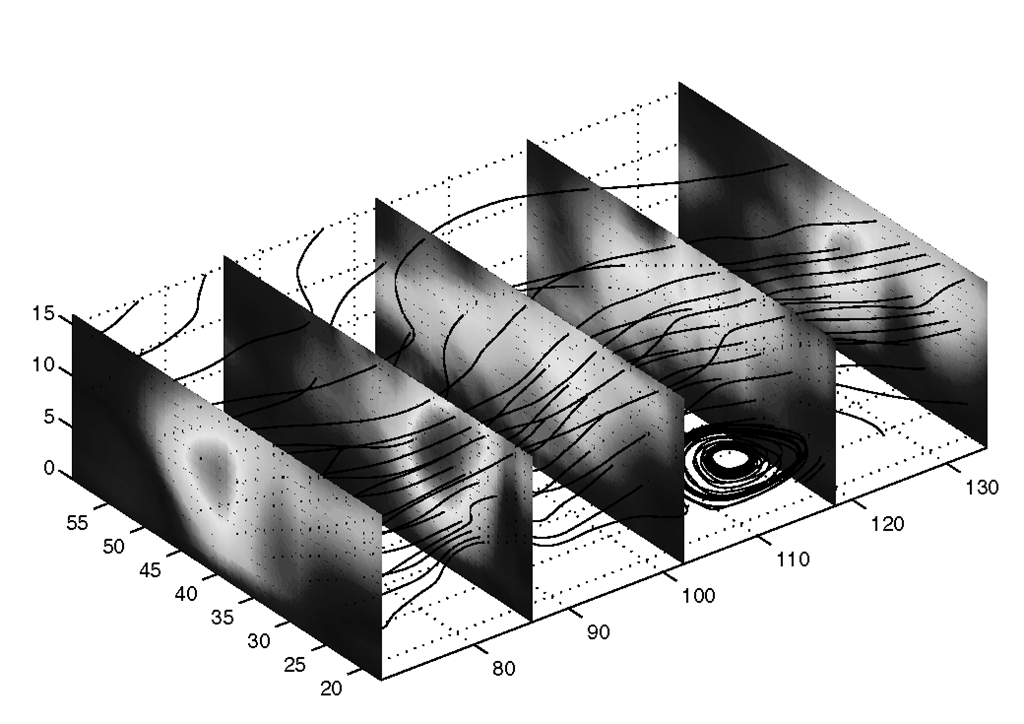
The other stream plotting function you should be familiar with is stream3. Refer to Table 4.3.2, for the form of the function. The wind data is almost ready for use by stream3, but we have to also provide starting points for the stream lines. The following example produces a plot much like Figure 4.44 but, rather than guessing, the limits of the volume are found using volumebounds. Five slice planes are located linearly spaced along the x-axis.

Next, meshgrid is used to define the start for the stream lines. The x-axis value is set to the lower limit of the volume, that will make all the stream lines start from the lower x -boundary. The y- and z-axis are incremented through their extents. (Yes, linspace could have been used here like it was with the slice function.)

Finally we use streamline to plot the result returned by the stream3 function.

The result is shown in Figure 4.46.

Figure 4.46 Stream lines with volume slices.

Stream Particles

Stream particles are used to put markers in the vector field. They can be used to show both position and velocity of the stream line. They are particularly useful in animation of stream lines.Here, we will deal with stream particles in the static case.

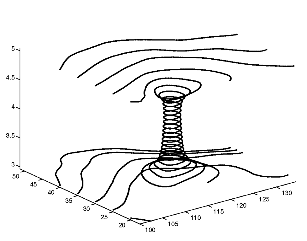
The function streamparticles relies on a variable called vertices which is a cell array that contains the vertices of the volume. This is the type of cell array that is typically returned by the stream3 function, and in fact, is what was used by streamline in the previous example. You can simply replace streamline in the previous example with streamparticles and MATLAB will reward you with success, but what you will see will look a bit messy. However, we can demonstrate using particles by noting that there is an interesting phenomenon between about 110 and 120 on the x-axis and between 15 and 40 on the y-axis. To investigate this area closer, we shall first redefine where we start our stream.

Then plot using streamline enhanced with streamparticles.

 

 

 

 

Figure 4.47 Stream particles combined with stream lines.

The string ‘markers’ is a keyword to streamparticles for "marker size" so that it will know that the number that follows specifies the size of the marker to use. Unfortunately, in this plot, the particles don’t convey any more information than the stream lines do.

Stream Ribbons

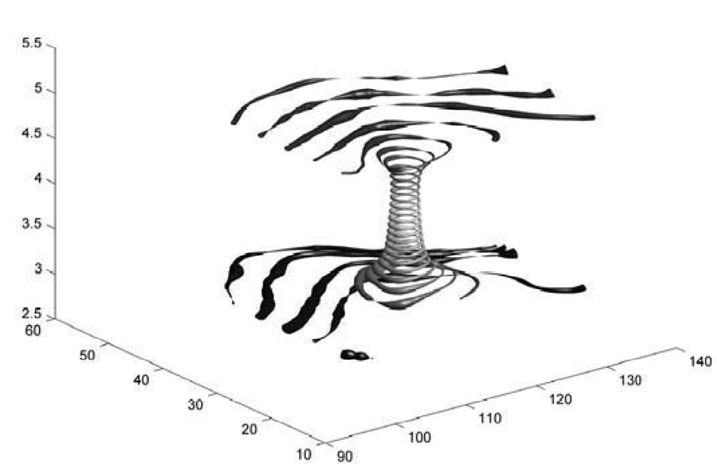
Stream ribbons are used to represent flow, just like a stream line, but unlike a line, a ribbon depicts the data direction and rotation about the axis of flow. This rotation is mathematically known as "curl" and we will not delve into the mathematical formulation for that here. If you know what curl is, then its use is obvious to you. If the concept of curl is new to you, you will find it most useful for vector field data such as that used in the example here. In this kind of visualization, the curl looks like a twist in the ribbon. In its basic form, the function streamribbon allows you to specify an angle for the twist for each vertex in the ribbon. However, streamribbon will determine the curl if you do not specify it. Note that the function curl is available for this type of computation.

The simplest way to use streamribbon is shown in the following code. Here, no twist is specified, so streamribbon will compute a twist proportional to the curl of the vector field. The width is constant and determined automatically. Figure 4.48 is the resulting plot.

 

 

 

Figure 4.48 Stream ribbons convey "twist" information.

As with other such plotting functions, streamribbon can return handles to the objects it creates. You are encouraged to read the helps on this function once you have read about Handle Graphics and Color and Light.

Stream Tubes

Since curl represents the "twist" about a vertex in vector fields, you might wonder what mathematical method is used to represent direction at each point, relative to the flow direction. This is called "divergence" and is most readily visualized with stream tubes that vary in diameter based on magnitude. The function streamtube is used much like streamribbon, and replacing the streamribbon function in the previous example with streamtube(x,y,z,u,v,w,sx,sy,sz) produces the plot shown in Figure 4.49 (see Plate 8).

Figure 4.49 Stream tubes are used to show divergence.

To better see the detail, you might zoom in on an interesting part of the plot as shown in Figure 4.50, or select a smaller subset of the volume.

Figure 4.50 A closer view of stream tubes reveals divergence.

Cone Plots

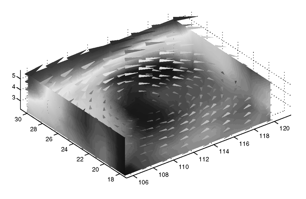
Cone plots represent the data in a vector field as a cone having direction and length proportional to the velocity at that point in the field. The function coneplot can be used to produce such a plot. As with the previous vector volume plots, you need to specify both the volume and volume vectors, but instead of just indicating where to start a stream, with coneplot you must specify the position of the cones within the volume.

Cone plots are very effective when combined with other volume visualization techniques. Using the wind data provided with MATLAB we will set about demonstrating using coneplot and introduce some new functions too. Consider the following code.

Here we use the function subvolume to extract only the portion of the volume we want to consider. Notice that the minimum y axis data is specified as NaN (Not-a-Number) which tells the subvolume function to start with the beginning of the data on that axis. As with our examples demonstrating stream lines, we find the wind velocity and this time make some slices at the boundaries of our data; the function volumebounds makes doing this convenient as it returns the extents of the volume in vector form. Now we specify the vertices where we want cones and pass those values to coneplot. Here we use coneplot in the form where we specify a matrix for color, in this case wind_vel. We also specify a comfortable size for the cones. The result is the plot shown in Figure 4.51 where the direction of each cone is the direction of the wind and both the length and color represent the velocity.

Figure 4.51 Cones visualize magnitude and direction in a vector volume field.