In This Chapter
Converting numbers among base systems
Converting values from one unit of measure to another
Finding the greatest common divisor and least common multiple
Generating random numbers with a twist
Advanced financial functions
Getting a fast set of statistics
Creating histograms
Working with moving averages
Creating a sample from a population
Just when you thought you had all of the Excel functions down pat, here we go rocking the boat. But in a good way. Excel ships with something called the Analysis ToolPak. This add-in provides several additional functions and dialog boxes that do cool things.
First start by getting that good old Analysis Toolpak loaded. Follow these steps:
1. Choose the Tools O Add-ins menu.
2. Check the check box for the Analysis Toolpak.
You can select all the add-ins you want, but for now this is all you need. The Analysis Toolpak-VBA provides a different set of functions than those from the standard Analysis Toolpak. In this chapter, we discuss the standard Analysis Toolpak.
3. Click the OK button.
If for any reason you do not see this add-in in the list, you need to speak to your network administrator, or call Microsoft, or call your uncle who is in the computer business.
Figure 20-1 shows the Add-ins dialog box where you select to use the Analysis
ToolPak.
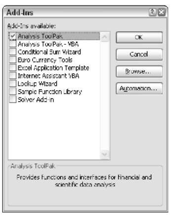
Figure 20-1:
Loading the Analysis ToolPak add-in.
Work with Hexadecimal, Octal, Decimal, and Binary Numbers
Base 2, base 8, base 10 — remember these from school? Here’s a refresher. In our daily lives, we work with numbers based on a system of 10 digits: 0, 1, 2, 3, 4, 5, 6, 7, 8, and 9. If you think about it, all numbers we put together consist of these digits. This is base 10, also called the decimal notation system, and it is based on powers of the number 10.
In certain lines of work, it is desirable or even necessary to work in another base system. Designing computer systems is a good example. The computer chips that run our PCs work with a binary system. Circuits are either on or off. This then means there are just two possible states — and they are often expressed as 0 and 1.
In base 2, or binary, all numbers are expressed with the digits 0 or 1. The number 20 as we know it in decimal, is 10100 in binary. The number 99 is 1100011. The binary system is based on powers of 2.
In other words, in base 10 you count up through 10 digits in one position before moving one position to the left for the next significant digit. And then the first position cycles back to the beginning digit. To make it simple, you count 0 to 9, and then add a 1 to the next significant digit, and start the first position over at 0, and therefore 10 comes after 9.
Binary, octal, and hexadecimal each count up to a different digit before incrementing the next significant digit. Binary only has two values — 0 and 1. That’s why when any larger base number, such as a base 10 number is converted to binary, there are more actual digit places. Look above at what happens to the number 20. In base 10, 20 is represented in 2 digits. In binary, 20 is represented 5 digits.
Octal, based on powers of 8, counts up to 8 digits — 0 through 7. The digits 8 and 9 are never used in octal. Hexadecimal, based on powers of 16, counts up to 16 digits, but how? What is left after 9? The letters of the alphabet, that’s what!
Hexadecimal uses these digits: 0, 1, 2, 3, 4, 5, 6, 7, 8, 9, A, B, C, D, E, and F. The letters A through F represent the decimal values 10 through 15 respectively. If anyone has ever worked on the colors for a Web site, you might know that FFFFFF is all white. The Web server recognizes colors represented in hexadecimal notation and responds appropriately.
Hexadecimal notation is used a lot with computers because the basic language of computers, which is binary, translates easily to hex (and vice versa). Each hex digit 0-F represents a 4-digit binary number, 0000 through 1111.
The number 200 in decimal notation becomes C8 in hexadecimal notation. The number 99 in decimal notation becomes 63 in hexadecimal notation.
Enough theory! The point to all this is that the Analysis ToolPak provides a group of functions to do all these conversions. These functions take into account all combinations of conversion between binary, octal, decimal, and hexadecimal. These functions are:
| Function | What it does |
| BIN2DEC | Converts binary to decimal |
| BIN2HEX | Converts binary to hexadecimal |
| BIN2OCT | Converts binary to octal |
| DEC2BIN | Converts decimal to binary |
| DEC2HEX | Converts decimal to hexadecimal |
| DEC2OCT | Converts decimal to octal |
| HEX2BIN | Converts hexadecimal to binary |
| HEX2DEC | Converts hexadecimal to decimal |
| HEX2OCT | Converts hexadecimal to octal |
| OCT2BIN | Converts octal to binary |
| OCT2DEC | Converts octal to decimal |
| OCT2HEX | Converts octal to hexadecimal |
You can find these functions in the Insert Function dialog box under the special Engineering category that appears when you load the Analysis ToolPak.
Convert Units of Measurement
CONVERT is a really great function that the Analysis ToolPak makes available. Not surprisingly it converts things, or more specifically it converts measurements. The number of measurements it converts is truly impressive. The function converts feet to inches, meters to feet, Fahrenheit to Celsius, pints to liters, horsepower to watts, and much more. In fact, there are 10 categories that contain dozens of units of measure to convert from and to. The categories are:
1. Weight and mass
2. Distance
3. Time
4. Pressure
5. Force
6. Energy
7. Power
8. Magnetism
9. Temperature 10. Liquid measure
The function takes three arguments: the value, the “from” unit of measure, and the “to” unit of measure. As an example, here is the function syntax for converting 10 gallons to liters: =CONVERT(10,”gal”, “l”). By the way the answer is 37.86.
See the Help topic for CONVERT to read all it can do. I’m sure you will find a use for it. In the meantime, Figure 20-2 shows a few conversions.
Can you use CONVERT to convert currency values, such as dollars to yen or pounds to marks? No — and the reason is because the conversion rate changes from day to day in response to economic factors.
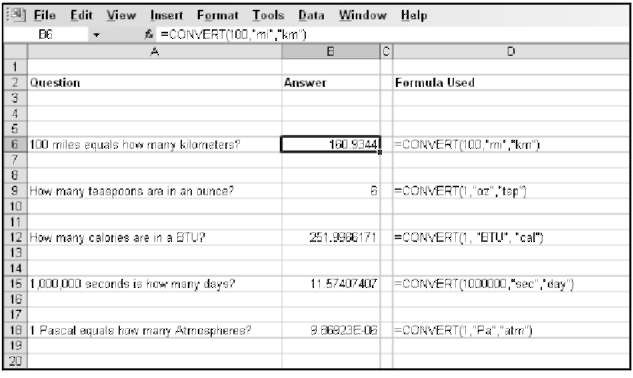
Figure 20-2:
Converting was never so easy!
Find the Greatest Common Divisor and the Least Common Multiple
A greatest common divisor is the largest integer that divides each number in a set of numbers and has no remainder after each division operation. Take the numbers 5, 10 , and 100. The greatest common divisor is 5, because each of the numbers divided by 5 returns another integer (no decimal portion).
The GCD function takes up to 29 values as its arguments. Non-integer values are truncated. By its nature any returned greatest common divisor must equal or be smaller than the lowest argument value. Often there in no greatest common divisor other than 1 — which all integers share. The syntax for the GCD function is:
![]()
The least common multiple is an integer that is the lowest multiple common among a group of integers. For example, the least common multiple of 2, 4, and 6 is 12. The least common multiple of 9, 15, and 48 is 720.
The LCM function takes up 29 values as its arguments. Non-integer values are truncated. The syntax for the LCM multiple function is:
Easy Random Number Generation
The Excel RAND function returns a real number between 0 and 1. And that’s it. Usually you have to massage the returned number into something useful. The typical thing to do is multiply it by some number to get it within a range of values, then add the lower limit to that, and then finally to use INT to turn the whole thing into an integer.
The days of drudgery are over. The Analysis ToolPak has a cool random number generation function that gives you the control you need.
The RANDBETWEEN function returns a random integer between two values. Two arguments are used — the low end of the range and the high end of the range. Just what we need! For example, =RANDBETWEEN(5, 10) returns a whole number between 5 and 10. Always.
Use Sophisticated Finance Functions
A collection of additional financial functions cover a variety of finance needs. Over 30 functions are provided that help with calculations in these broad areas:
Accrued interest, cumulative interest, nominal interest Depreciation
Coupons (the securities kind, not the ones for the supermarket!)
Converting dollar amounts into decimals and fractions
Price and yield for securities with an odd first period or odd last period
Price and yield for Treasury bills
Price and yield for other securities
If you work in the field of high finance, you will surely find some of these useful.
Generate Descriptive Statistics
You have a set of data. You need to calculate the mean, the standard deviation, and other statistical measures. Well, you can enter all the necessary functions yourself and get the answers. To be honest this may very well be preferable regardless of what we are about to show you. Perhaps you need the mean in a certain cell, the standard deviation in another dedicated place, and so on.
But if you are not that particular, then the Analysis ToolPak has just the thing for you. After the ToolPak is loaded, you find a new sub-menu item, Data Analysis, under the Tools menu.
Using the Tools O Data Analysis menu displays the Data Analysis dialog box, shown here in Figure 20-3.
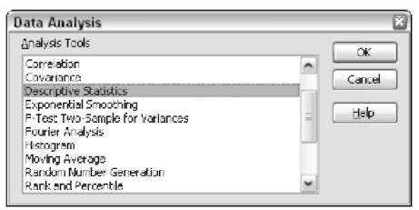
Figure 20-3:
Displaying the Data Analysis dialog box.
One of the choices in the dialog box is Descriptive Statistics. Selecting that brings up the Descriptive Statistics dialog box, shown in Figure 20-4.
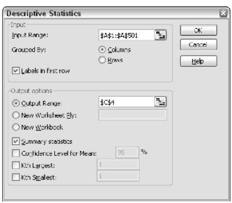
Figure 20-4:
Making selections about which statistics to return.
In this dialog box, you enter the range of the source data, the location where to display the results, and which results to display. The statistical calculations are done for you. You select how much to display. There is a basic set of statistics, but also a few extras, such as the confidence level, can be generated as well. Figure 20-5 shows the results of selecting the basic summary statistics. You could create this result with individual Excel functions but the Analysis ToolPak makes it a lot easier.
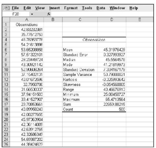
Figure 20-5:
A returned set of descriptive statistics.
Even though the Descriptive Statistics feature returns a wealth of statistical data, the results are returned as values, not formulas. Any changes to the source data are not reflected in the results. You need to regenerate the statistics.
Create a Histogram
A histogram is a set of counts within ranges — in other words, how many of your values fall into each range. The ranges are called bins. Making a histogram is easy with the Histogram dialog box, shown in Figure 20-6. You display this dialog box by selecting it in the Data Analysis dialog box shown earlier in Figure 20-3.
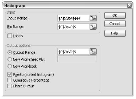
Figure 20-6:
Defining a histogram.
A histogram requires the range of the source data, the range of the bin designations, and where to place the output. The returned bins and counts make it easy to show the distribution of data. Figure 20-7 shows the histogram created with the parameters seen in Figure 20-6.
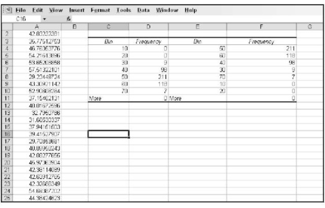
Figure 20-7:
A histogram shows the distribution of data.
Histograms often serve as the source for a chart. One of the options in the Histogram dialog box is to have a chart generated along with the data.
Generate Moving Averages
Moving averages help identify trends in sequential data. The data is period based, such as on a daily basis, and an average is calculated for a number of
periods. Then the average is rolled through the data. So the first average may be for days 1 through 7, then the next average is for days 2 through 8, and so on.
One of the selections in the Data Analysis dialog box, shown in Figure 20-3, is Moving Average. Choosing this brings up the Moving Average dialog box, shown in Figure 20-8.
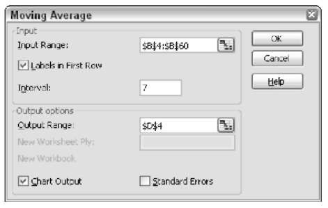
Figure 20-8:
Selecting parameters to create a moving average.
In the Moving Average dialog box, you select the range of the source data, the interval step, and the output range. The interval step is a key component. In this example, we selected 7 as the interval. Because the data is daily, this creates a 7 day, or weekly, moving average. One of the output options is to create a chart, which is selected in this example. Figure 20-9 shows the output.
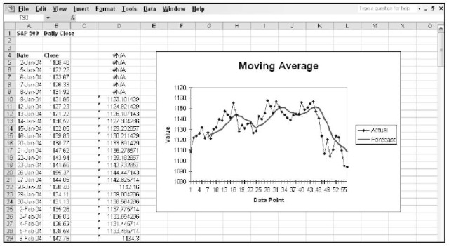
Figure 20-9:
Moving average values and a chart to boot!
Cell D4 had been selected for where the output should start. Notice that the first six cells starting from D4 do not return a useful value. This makes sense because it takes at least seven values to make an average. Therefore the first usable average is in cell D10, with this formula: =AVERAGE(B5:B11). Cell D11 has this formula: =AVERAGE(B6:B12). Cell D12 has this formula: =AVERAGE(B7:B13).
Moving averages are used to diminish the effects of spikes in data and to identify trends. Viewing a plot of raw value points can seem random and chaotic. Viewing a moving average of the data set removes some of the volatility and hopefully shows a line with a sense of direction. The chart in Figure 20-9 shows two series lines — the source data (labeled as Actual) and the moving average (labeled as Forecast). The moving average smoothes out the spikes and provides a cleaner view of movement.
Advanced Random Number Generation
One of the selections in the Data Analysis dialog box, shown in Figure 20-3, is Random Number Generation. Choosing this brings up the Random Number Generation dialog box, shown in Figure 20-10.
Excel has the plain RAND function, the Analysis ToolPak has the RANDBE-TWEEN function, and here is yet another way to make random numbers. There must be something special about them!
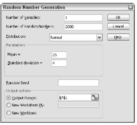
Figure 20-10:
Mucho control over random numbers.
The Random Number Generation dialog box is quite advanced compared to the two random number functions. Whereas the functions just generate numbers within a range, here you have much more control:
Number of Variables: The number of columns of data to return.
Number of Random Numbers: How many values to return, per column.
Random Seed: An optional value from which to generate numbers. Using this number in another session returns the same random values.
In the middle of the dialog box is a drop-down list from which you select the distribution type, and below it are the parameters. The type of parameters change which each type of distribution:
| Distribution Type | Parameters |
| Uniform | low value and high value |
| Normal | mean and standard deviation |
| Bernoulli | p value |
| Binomial | p value and number of trials |
| Poisson | lambda |
| Patterned | low value, high value, step, number of repeats |
| Discrete | value and probability |
Create a Random Sample
One of the selections in the Data Analysis dialog box, shown in Figure 20-3, is Sampling. Choosing this brings up the Sampling dialog box, shown in
Figure 20-11.
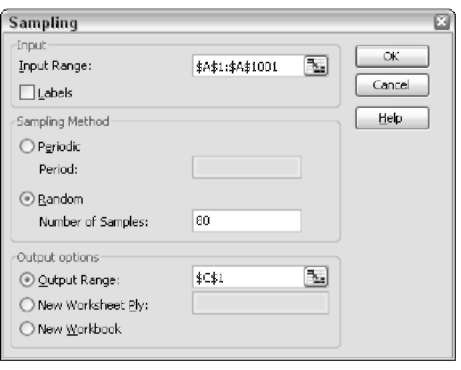
Figure 20-11:
Pulling a sample from a population.
Statistical analysis is often done on a sample of data from a population, instead of the population itself. For example, you may have 20,000 observations of a periodic temperature reading and decide to use a portion of the data to run analysis.
The Sampling dialog box takes an input of where the source population data is, and where the sample data should be placed. You also select a setting for how the sample data is pulled out of the population. When the sampling method is periodic, you supply the step pattern. When the sampling method is random, you supply the number of values to return. The Sampling dialog box is a real timesaver. You can generate a sample instantly instead of hunting and pecking through the population data.
