Adaptive Filtering (Image Processing) Part 2

Adaptive Image Filtering in MATLAB

The imnoise function in the Image Processing Toolbox can be used to add speckle noise to an image by passing in the string ‘speckle’ and the noise variance as input arguments to the function. Note that the noise variance argument in this sense is not the same as <x„2 – in this context it is used to scale a zero-mean uniform distribution of variance 1 to produce noise of the desired magnitude. Obtaining the a„2 parameter used in the MMSE, adaptive local noise reduction, and SAM filters requires looking at the variance of pixel intensities of a noisy background portion of the image, or estimating it through means that shall be discussed shortly.

The MATLAB function uses a slightly different model for corrupting an image with multiplicative speckle noise than what was previously described.

Other models, some of which simulate the noise using a Rayleigh distribution, are also common for modeling speckle noise. Listing 4-14 is a replacement for imnoise (when used with the Speckle’ argument), which can be used if the Image Processing Toolbox is not available or if a different model for speckle noise is desired.

Listing 4-14: MATLAB function for corrupting an image with multiplicative speckle noise.

The Image Processing Toolbox provides a function wiener2 (see Figure 4.24c) that implements an adaptive filter of the form

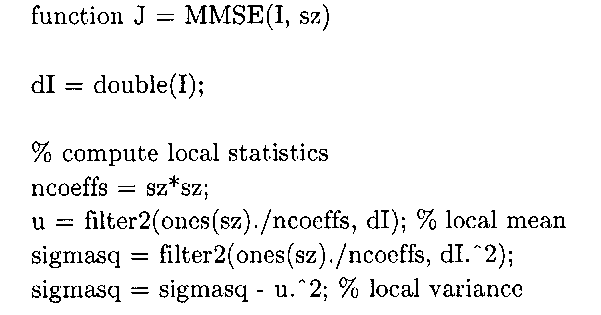
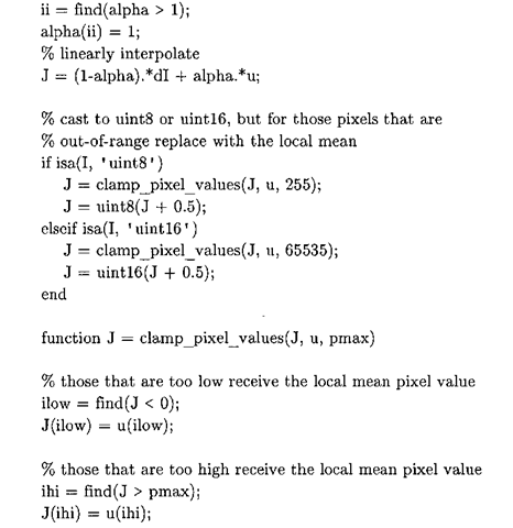
This particular filter is very well-suited to the removal of additive noise. Listing 4-15 is an M-file that implements Algorithm 4-2, the MMSE filter. MMSE uses the built-in MATLAB function f ilter2 to compute the local means and local variances. After these temporary matrices have been constructed, the code proceeds to implement the core MMSE algorithm in classic vectorized MATLAB form.

Listing 4-15: MATLAB function for passing an image through the MMSE filter.

% from the local variances estimate the noise variance noise_variance = mean2(sigmasq);

% the guts of the MMSE adaptive filter

% (linearly interpolate b/w input pixel and local mean,

% depending on the magnitude of the local variance) alpha = noise_variance ./ sigmasq;

% must be careful to handle the case where noise variance

% much greater than local variance – in this case the output

% pixel should be the local mean (alpha = 1)

One of the drawbacks to adaptive image filtering, aside from increased computational complexity, is the presence of various parameters for tuning the image processing. While these algorithm constants are certainly useful for tweaking the processing, in the case of the ubiquitous noise variance parameter it is generally difficult to obtain this measurement without resorting to less-than-ideal techniques. One course of action is to simply disregard the question entirely, and leave it up to clients to provide a meaningful number, perhaps by extracting a representative background area containing nothing but noise, and computing the variance of this training data beforehand. The MMSE implementation of Listing 4-15 does not expect clients to provide the noise variance – rather, the noise variance is estimated from the input data by calculating the noise "power" from the mean of all the local variances. Strictly speaking, while this estimation is meant for additive noise, it does work adequately in the presence of multiplicative noise, and therefore can be used to despeckle images. This technique is used for all of the adaptive filtering code in this topic whenever an algorithm calls for <j„2.

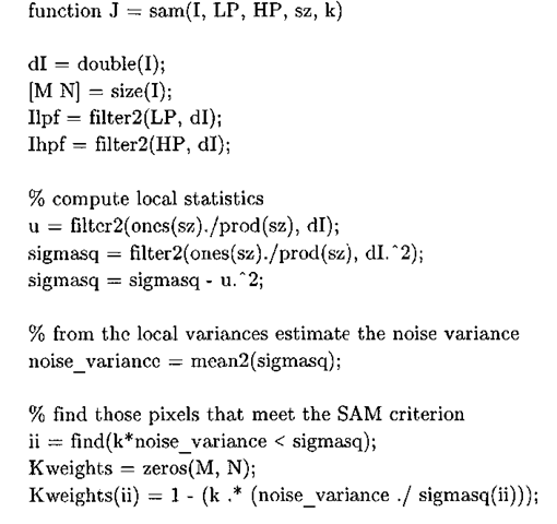
Listing 4-16 is a MATLAB implementation of the SAM filter. This function again uses filter2to compute thematrices (u and sigmasq, respectively) as before, but also uses f ilter2 to pass the input image through low-pass and high-pass filters, whose kernels are function arguments to SAM. The find function is then used to demarcate those pixels that meet the criterionand these pixels, whose indices are given by the i i vector, are then replaced by a linear weighting of the low-pass and high-pass pixels. A final processing step is to clamp the pixel intensities to a range appropriate for the data type of the input image.

Listing 4-16: Signal Adaptive Mean (SAM) MATLAB function.

 

 

 

 

An MMSE Adaptive Filter Using the Intel IPP Library

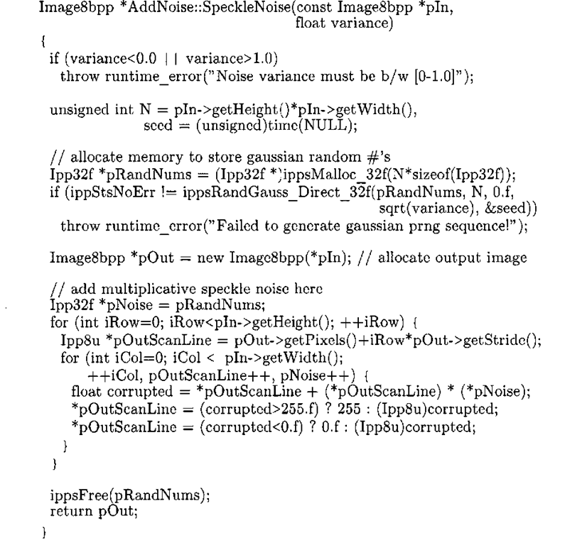
The Intel Integrated Performance Primitives library actually consists of three APIs: the image processing component we have dealt with exclusively up until now, a component for one-dimensional signal processing, and a suite of basic mathematical functions for matrix math. The application described here is the first program that uses functionality from the signal processing component, and can be found in the Chap4\ AdaptiveFilter\MMSE_VS directory. The application’s interface is very similar to that of the program discussed in 4.5.4, but instead of querying the user to enter in the percentage of shot noise, there is an edit box for the user to enter the noise variance of the multiplicative speckle noise. The project links to the Intel IPP Signal Processing static library ipps20 . lib and includes the signal processing library header file ipps . h, in addition to the usual IPP Image Processing dependencies. The AddNoise class has been updated with a new method SpeckleNoise (given in Listing 4-17) that uses ippsRandGauss_Direct_32f and ippsMalloc_32f from the Intel Signal Processing Library to generate Gaussian random variables which are subsequently used to contaminate input pixels with multiplicative speckle noise. The ippsRandGauss_Direct_32f function requires a mean and standard deviation to generate the Gaussian distribution. Because the user is prompted to enter in the noise variance on the main application window, the square root of this input parameter is then passed into ippsRandGauss_Direct_32f, and then this distribution is multiplied by the image data in a pixel-wise form, thereby simulating a speckled image.

Listing 4-17: AddNoise: : SpeckleNoise

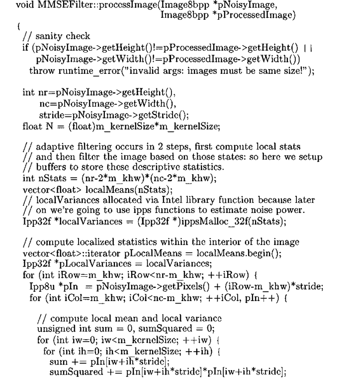
The MMSEFilter class is at the heart of this application, and its implementation is given in Listing 4-18. This code is somewhat unoptimized (for example, there are Intel IPP functions to compute pixel statistics) but the goal here is provide a starting point, as there are quite a few issues that need to be addressed when porting this algorithm on to the DSP. Essentially, this implementation of the MMSE algorithm proceeds in two phases and this general structure will be carried over in the DSP implementation. If the noise variance is known in advance, then the two phases could be collapsed into one, which should result in a performance boost. However, MMSEFilter does not require clients to know the noise variance, and as a consequence the first phase, which consists of a quadruple loop, entails computing the localized statistics of the image for each neighborhood. In between the two phases, the noise variance is estimated using the same technique as the MATLAB implementation, and then during the second phase we march through the image, replacing pixels if they meet the MMSE criterion.

Listing 4-18: The MMSEFilter class.