Warnock and Weiler-Atherton Area Subdivision
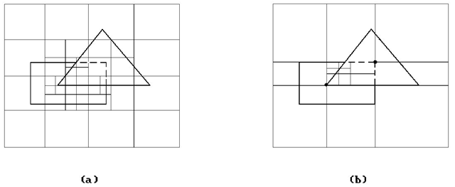
The Warnock visible surface determination algorithm [Warn69] is an image space algorithm that attempts to find rectangular regions (here called windows) of the same intensity on the screen (area coherence). Algorithm 7.6.1 is an outline of the algorithm. The polygons referred to in the algorithm are the projected polygons. See Figure 7.5.
Essential to this algorithm is the ability to perform the following tests on any polygon P:
Algorithm 7.6.1. Outline of the Warnock algorithm.
Figure 7.5. Area subdivision examples.
Test 1: Is P disjoint from a window?
Test 2: Does P surround a window?
Test 3: Does P partially meet a window?
Test 4: Does P fall inside a window?
Test 5: Is P in front of other polygons?
For a quick test for disjointness, one usually uses bounding boxes. One way to test if the window falls inside a polygon is to substitute the vertices of the window into the equations for the edges of the projected polygons. If these tests fail, then one needs to check if the boundary of the polygon intersects the window by checking each edge of the polygon against each edge of the window. If the boundaries are disjoint, then one still has to distinguish between the case where the regions are disjoint or where one contains the other. We discussed some tests for doing this in Section 6.3. One approach is to use a parity test and count the number of times that, say, any horizontal ray starting at a window vertex intersects the polygon. If the number is even, then the two are disjoint, otherwise the polygon surrounds the window. Another approach is to use an angle counting argument.
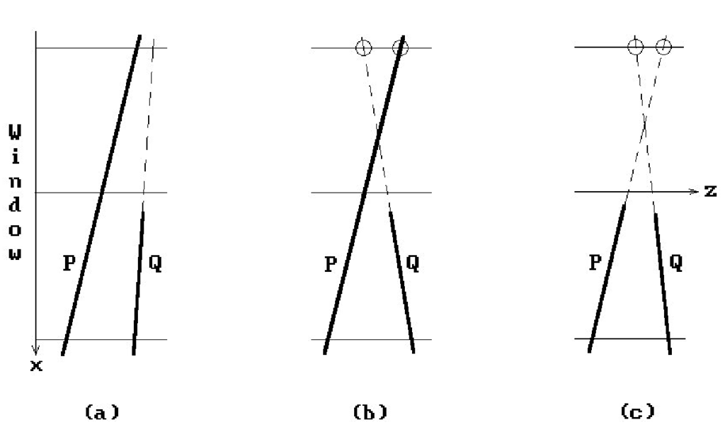
Tests 1-4 above dealt with view plane issues. Test 5 involves depth calculations. As mentioned earlier, we are assuming an orthogonal projection (with the camera at -•) and so testing if one point is in front of another amounts to checking that its z-value is less than that of the other point. Assume that two polygons P and Q meet the window. We give a test for whether P is in front of Q. In Warnock’s algorithm this test is only needed for the case P is a surrounding polygon, but the fact that it is surrounding is not important. Here is the test: if the depth of the plane of P is less than the depth of the plane of Q at the four corners of the window, then P is in front of Q (Figure 7.6(a)). This is a sufficient but not necessary condition for that to happen (Figures 7.6(b) and (c)). Warnock subdivides the window if the test fails.
There are many variations of Warnock’s algorithms. The windows need not be rectangular. The problem with rectangular windows is that, being bad matches to most polygons, the algorithm has to recurse down to the pixel level a lot. The Weiler-Atherton algorithm ([WeiA77]) uses subwindows that match the shape of the polygons. See Figure 7.7, which shows a list of polygons being clipped against a polygon P. The resulting pieces are separated into two lists, those that lie inside P and those that lie outside. This is more complicated to implement and the authors had to develop a new clipping algorithm, which was discussed briefly in Section 3.3.2, but it is more efficient.
Figure 7.6. Examples of a face in front of another face.
Figure 7.7. Weiler-Atherton type area subdivision.
Both the Warnock and Weiler-Atherton algorithms are not scan line oriented but jump around as they draw the scene. Their complexity is approximately the complexity of the final display (not of the scene).
Z-buffer Algorithms
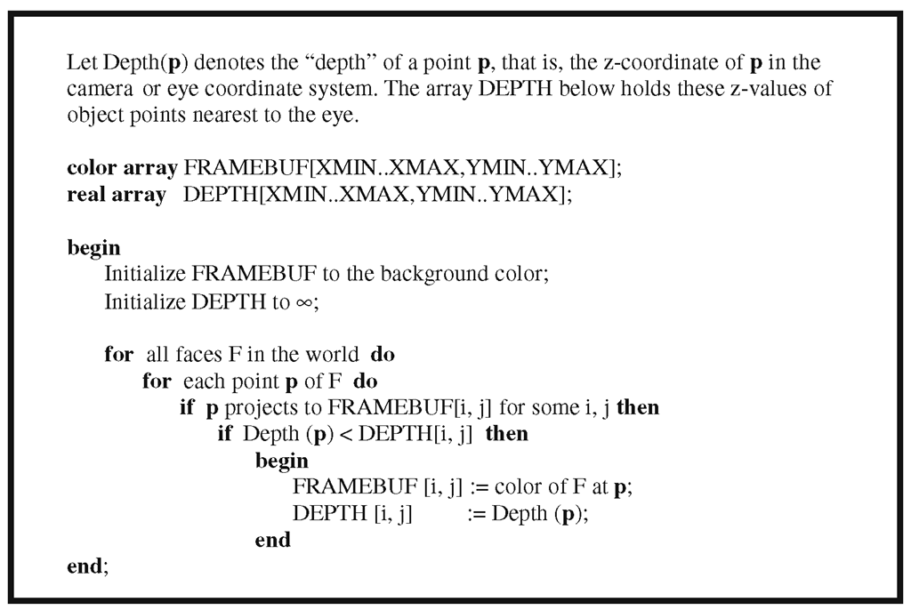
Z-buffer algorithms record "current" depth information for each pixel. A "real" Z-buffer is a two-dimensional array of real numbers of the same size as the frame buffer. The real numbers record current depth information. A Z-buffer algorithm then scan converts an entire face at a time into both the frame and the Z-buffer. The high-level outline of such algorithms is extremely simple and is shown in Algorithm 7.7.1. There are variants of the Z-buffer algorithm that incorporate antialiasing. An early scan line approach described in [Catm78] was computationally expensive. A more efficient approach, called the A-buffer algorithm, is described briefly in Section 7.11.
Algorithm 7.7.1. The Z-buffer algorithm.
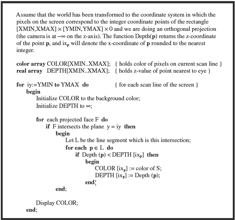
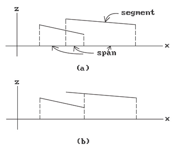
A Z-buffer takes up a lot of memory. By taking a scan line approach, one only needs an array as long as a scan line. This leads to a slightly modified Z-buffer algorithm shown in Algorithm 7.7.2. See [Roge98]. Such Z-buffer algorithms all use the notion of “segment” and “span” in a scan line (where a face intersects the scan line) and ask the question “Which segments are visible?” One uses the x-z plane. The dotted lines in Figure 7.8(a) divide the scan lines into “spans.” Within each span one determines the visibility of segments by checking their depths using plane equations. Different choices of spans are possible because the only criterion is that one can unambiguously order the segments within it by their depths. Therefore, there is the issue of how to best choose the spans? For example, Figure 7.8(b) shows a better choice of spans than Figure 7.8(a).
The scan line algorithms all do
(1) a Y sort to limit attention of algorithm to edges or faces which intersect scan line
(2) an X sort
(3) Z depth search
With regard to (1), one brings in new edges, etc., as one proceeds to the next scan line and discards those that are no longer needed. One uses coherence and a list of “active” edges.
Algorithm 7.7.2. A scan line Z-buffer algorithm.
Figure 7.8. Z-buffer spans.
For (2) one divides the scan line into "sample spans" within which the same face is visible (one is using "point-to-point" coherence along the line). Finally, at step (3) each sample span must then be processed. How this is done depends on how they were chosen. If we use the method indicated in Figure 7.8(a), then this is straightforward, although if we allow penetrating faces there are extra modifications needed: At each vertex or span endpoint one must compute the depths of the segments that fall into the span.
The Watkins Scan Line Algorithm
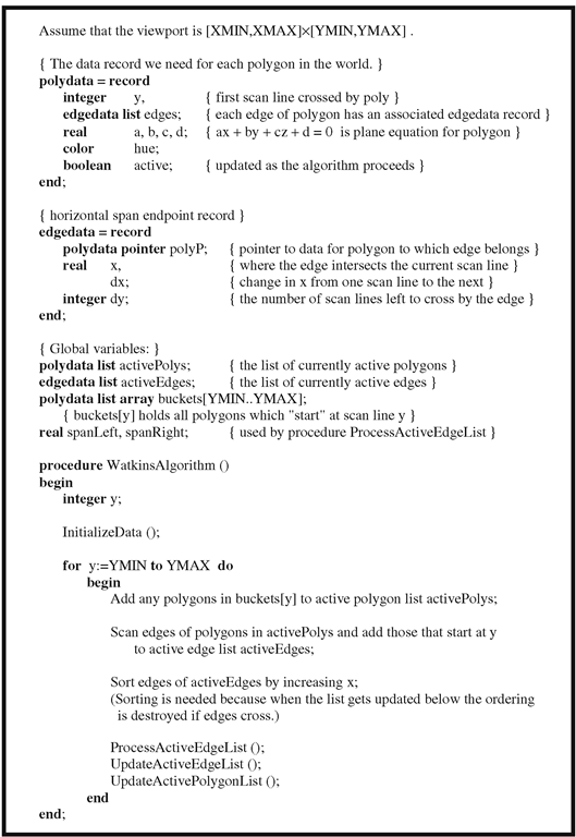
The Watkins algorithm ([Watk70]) is a scan line image space algorithm that is especially efficient. The idea is to let the right end of the current span "float" and keep the left end fixed. One starts at the extreme right. As new segments are taken from the x-sorted list, the right end moves left until one gets a span that is simple enough to compute which segment is visible.
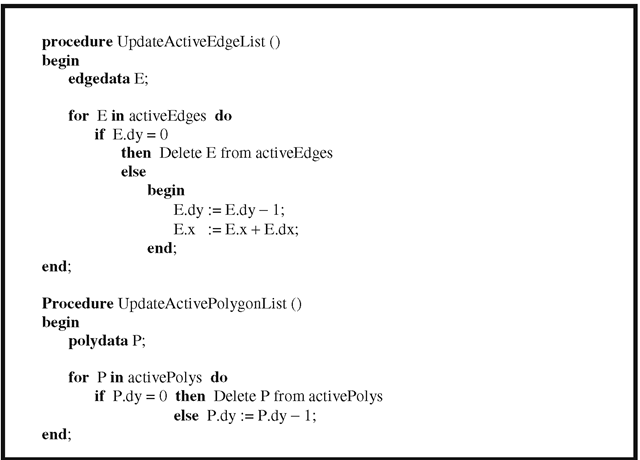
Algorithm 7.8.1 gives an outline of a Watkins-type algorithm. There are two things to note. One is that for parity to work, one needs to shorten the edges appropriately as described in Section 2.9.1. The other is that we assume that polygons have been clipped.
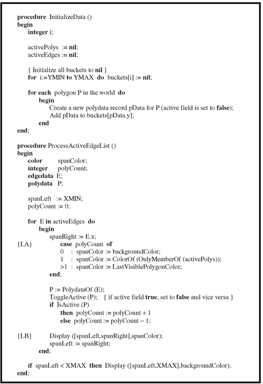
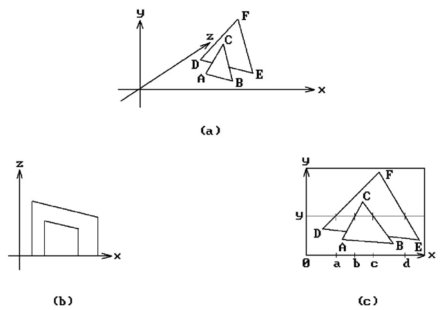
To help clarify the algorithm we shall work through an example. Consider the scene shown in Figure 7.9(a). Figures 7.9(b) and (c) show its projection onto the x-z and x-y plane, respectively. Suppose that we are at scan line y as shown in Figure 7.9(c). The critical points along the x-axis are 0, a, b, c, and d. Table 7.7.1 shows how the x scan progresses. We show the values of the indicated variables at the locations in the procedure ProcessActiveEdgeList marked "LA" or "LB." Note how the active flag for each polygon toggles back and forth between true and false based on a parity-type argument.
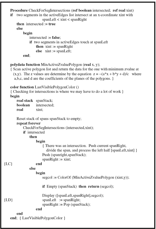
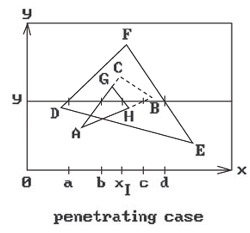
The objects in Figure 7.9(a) did not intersect. Figure 7.10 shows a case where one polygon penetrates another. In such a case we have to find intersections and keep moving the right end of the span to the left, saving the current values as we go along, until we find an intersection-free segment. In the case shown there is one intersection with x value xi in the segment [b,c]. We need to check all active polygons against all other active polygons when testing for intersections. We can tell if two polygons intersect by looking at their z-depth values at the endpoints of the span, call these zl1,zr1 for the first polygon and zl2,zr2 for the second polygon. The polygons will intersect if
If we find an intersection, then certain branches in the code of the procedure LastVisiblePolygonColor will now be executed. The new x scan will now pass statements marked "LC" and "LD," as we can see from Table 7.7.2 in our example. First we save c on the stack and deal with the segment [b,xI]. Then we set spanLeft to xI, pop c from the stack, and deal with [xI,c]. The rest proceeds as before.
Notice that we always check if segments intersect in an endpoint of a span. If so, then we use the opposite endpoint’s x value to do a depth check to see which polygon is closer.
Algorithm 7.8.1. A Watkins visible surface algorithm.
Algorithm 7.8.1. A Watkins visible surface algorithm.
Algorithm 7.8.1. A Watkins visible surface algorithm.
Algorithm 7.8.1. A Watkins visible surface algorithm.
Figure 7.9. A Watkins scan line algorithm example.
Table 7.7.1 The x-scan data at scan line y for Figure 7.9(c).
|
Label |
polyCount |
span Left |
spanRight |
ABC.active |
DEF. active |
|
LA |
0 |
0 |
a |
F |
F |
|
LB |
1 |
0 |
a |
F |
T |
|
LA |
1 |
a |
b |
F |
T |
|
LB |
2 |
a |
b |
T |
T |
|
LA |
2 |
b |
c |
T |
T |
|
LB |
1 |
b |
c |
F |
T |
|
LA |
1 |
c |
d |
F |
T |
|
LB |
0 |
c |
d |
F |
F |
Figure 7.10. The Watkins scan line algorithm with penetrating objects.
Table 7.7.2 The x-scan data at scan line y for Figure 7.10.
|
Label |
polyCount |
spanLeft |
spanRight |
ABC.active |
DEF. active |
spanStack |
|
LA |
0 |
0 |
a |
F |
F |
nil |
|
LB |
1 |
0 |
a |
F |
T |
nil |
|
LA |
1 |
a |
b |
F |
T |
nil |
|
LB |
2 |
a |
b |
T |
T |
nil |
|
LA |
2 |
b |
c |
T |
T |
nil |
|
LC |
2 |
b |
XI |
T |
T |
c |
|
LD |
2 |
xi |
c |
T |
T |
nil |
|
LB |
1 |
xi |
c |
F |
T |
nil |
|
LA |
1 |
c |
d |
F |
T |
nil |
|
LB |
0 |
c |
d |
F |
F |
nil |

