Raster Algorithms (Basic Computer Graphics) Part 2

Fill Algorithms

Contour-filling algorithms are used in many places. For example, in pattern recognition problems integrals may have to be computed over areas; in photo typesetting, fonts are described by contours that are later filled; in animation, the cel painter who fills figures has the next most time-consuming job after the animator.

There are two broad classes of such algorithms – polygon-based (edge-filling) algorithms and pixel-based algorithms. The former can be used in the case where the regions to be filled are defined by polygons and we can use the equations for the edges. The latter are, in a sense, more general because they can be used both for polygonal regions and also arbitrary regions whose boundaries are defined on the pixel level.

There is also a distinction as to how the algorithm decides whether a point is in the interior of a region. Some use a parity check that is based on the fact that lines intersect a closed curve an even number of times (if one counts intersections at certain special points such as at points of tangency correctly). This test is always used in case of polygon-based algorithms, but can also be used for pixel-based ones. Other algorithms, called seed fill algorithms, use connectivity methods. Here it is assumed that one is given a starting point or seed. Then one sees which pixels can be reached from this one without crossing the contour. The bounding curves can be quite general. This approach applies only to pixel-based algorithms. Also, one needs to know an interior point. This is okay in interactive situations (where one picks one using a mouse, for example), but if one wants to automate the process, note how border-following algorithms become relevant.

In this section we shall describe the pixel-based seed fill algorithms. Section 2.9.1 will look at polygon-based fill algorithms.

The Flood Fill Problem: Given distinct colors c and c’, a set A of the same color c bounded by points whose colors are different from c and c’, find an algorithm that changes all points of A and only those to the color c’.

An algorithm that solves this problem is called a flood fill algorithm. There are a number of related fill problems and associated algorithms. For example, boundary fill algorithms assume that all points of the boundary have the same color, which is dif- ferent from the color inside the region, where the boundary of a set S means here the set of points of Sc that are adjacent to S.

Algorithm 2.4.1. The basic fill algorithm.

In the algorithms of this section, the Boolean-valued function Inside(x,y) determines whether or not the pixel at (x,y) has the property one wants. The procedure Set(x,y) sets the value of the pixel at (x,y) to its desired value. For example, to get a flood fill algorithm let Inside(x,y) be true if the value of the pixel at (x,y) agrees with the value of the pixels in the region and let Set(x,y) set the pixel value to its new value (the same as Draw(x,y,c’)). Using the functions Inside and Set will make our algorithms more general and applicable to a variety of fill algorithms. There is one constraint on the Inside function however: Inside(x,y) must return false after an operation Set(x,y).

Assume 4-adjacency is chosen and that our regions are 4-connected. The BFA procedure in Algorithm 2.4.1 shows that the basic idea behind a fill algorithm is very simple. Notice that 4-connected is important and that the algorithm will not work if the region is not 4-connected.

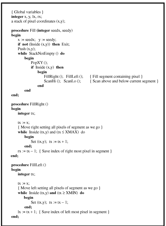
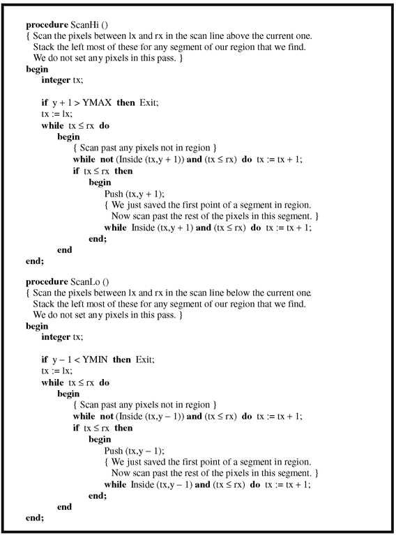
Although the BFA algorithm is simple, the recursion is expensive. One of the earliest nonrecursive algorithms is due to Smith ([Smit79]). It is not very efficient because pixels are visited twice, but many of the better algorithms are based on it. It will be worthwhile to describe Smith’s algorithm, Algorithm 2.4.2, first before we present the one due to [Fish90b]. In this algorithm and the next, the constants XMIN, XMAX, YMIN, and YMAX define the minimum and maximum values for the x- and y-coordinates of pixels in the viewport. The procedures Push and Pop push and pop a pair (x,y) onto and from a stack, respectively. The function StackNotEmpty tests whether this stack is empty or not. The procedures Inside and Set are as described above.

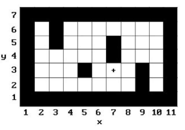
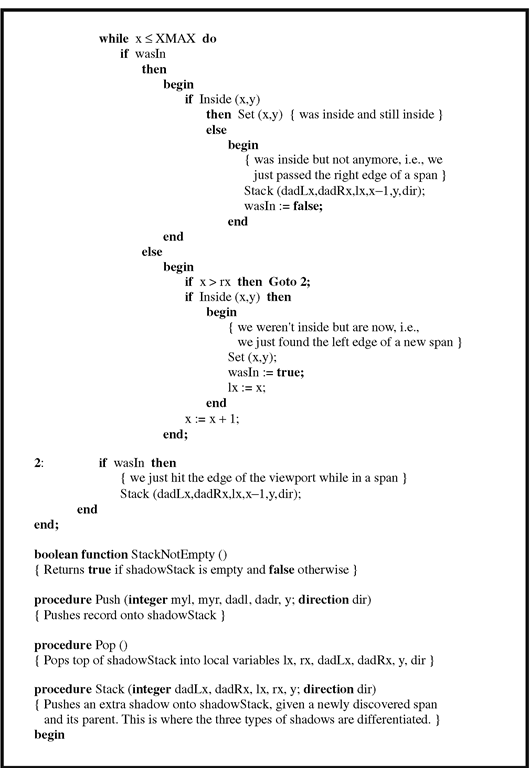
For example, suppose that in Figure 2.5 our starting point is (7,3). After the first FillRight command the two-pixel segment from (7,3) to (8,3) would have been filled. The FillLeft command would fill (6,3). The ScanHi command would place the pixel coordinates (6,4) and (8,4) on the stack in that order. The ScanLo command would add (6,2). The segments of the region that (6,4), (8,4), and (6,2) belong to are usually called “shadows.” The point of the ScanHi and ScanLo procedures is to find these shadows that still need to be filled. We now return to the beginning of the main while loop, pop (6,2), and make that our new starting point. The next FillRight and FillLeft would fill the segment from (2,2) to (8,2). The ScanHi and ScanLo would put (2,3) and (6,3) on the stack. The loop would start over and pop (6,3). This time, since (6,3) has already been filled, we immediately jump back to the beginning and pop (2,3), and so on.

Algorithm 2.4.2. The Smith seed fill algorithm.

Algorithm 2.4.2. The Smith seed fill algorithm.

Figure 2.5. A fill algorithm example.

Figure 2.6. Pixel shadows. 

The problem with Smith’s basic algorithm is that we look at some pixels twice, as we saw in the case of (2,3) in the previous example. This happens because we automatically put coordinates from both the line above and the line below the current one on the stack. When we then, say, deal with the line above, the algorithm will have us look at the current line again because it will be the line below that one.

An alternative improvement to Smith’s seed fill algorithm is described by Heck-bert in [Heck90b].

Finally, another distinction that is made between flood fill algorithms is whether we are dealing with hard or soft area flooding. The algorithms we have described so far were hard area flooding, which basically assumed that the region to be filled was demarcated by a “solid” boundary, that is, a curve of pixels all of the same color. Such a boundary would be a jagged curve. To get a smoother looking boundary one typically would blur or “shade” it by assigning a gradation of colors in a neighborhood of it. (The causes of the “jaggies” and solutions to the aliasing problem are discussed later in Section 2.6.) If boundaries are shaded, then we would like filling algorithms to maintain this shading. Soft area flooding refers to algorithms that do this and leave any “shading” intact. Smith’s paper [Smit79] is a good reference for both hard and soft area flooding. The tint fill algorithm he describes in that paper is a soft area flooding algorithm.

There are other types of pixel-based fill algorithms. Pavlidis [Pavl82] describes a parity check type algorithm. Rogers [Roge98] describes various algorithms for filling regions bounded by polygons that he calls “edge fill” algorithms.

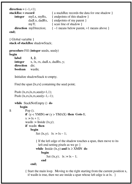
Algorithm 2.4.3. The Fishkin seed fill algorithm.

Algorithm 2.4.3. The Fishkin seed fill algorithm.

Algorithm 2.4.3.The Fishkin seed fill algorithm.

Generating Discrete Curves

Now we start a central topic of this topic, namely, curves and the problem that one runs into when one tries to represent them with a discrete set of points. Clearly, we want any mapping of continuous structures into discrete ones to preserve the visual shape properties, such as smoothness and uniform thickness, as much as possible but this is not easy. We shall look at the problem of defining and generating discrete lines first and then conics.

Lines, or more accurately segments, are the most basic of computer graphics objects because most modeling systems use linear approximations to all objects so that displaying them reduces to drawing lots of lines. It is possible to actually give a formal definition of a discrete “straight” line (see [ArcM75] and [BoLZ75]). Not surprisingly, such definitions get complicated, but from a practical point of view we are not really interested in a definition. Rather, we are happy with an algorithm that generates a satisfactory set of points for a line. What is satisfactory? Well, that is not very precise, but some attributes that we want the generated discrete lines to have are:

(1)  Visually, the line should appear as straight as possible.

(2)   The line should start and end accurately, so that, for example, if several contiguous line segment are drawn, then there is no gap between them.

(3)  Each line should appear to have an even visual thickness, that is, it should have as constant a density as possible, and this thickness should be independent of its length and slope.

(4)  The conversion process must be fast.

In Sections 2.5.1-2.5.3 we look at line-drawing algorithms for the monochrome case, that is, where the raster is an array of 0′s and 1′s and the line consists of those pixels that are set to 1. Section 2.6 looks at some deeper problems that one encounters in the process of discretizing continuous objects and making them look smooth. Section 2.9.1 looks at a scan line algorithm for lists of lines and fill algorithm for polygons.

Conics are the next most common curve after the “straight” line. The circle is one obvious such curve, but the other conics are also encountered frequently. Their geo metric properties and relatively low degree (when compared with the popular cubic splines) make them attractive for use in designing shapes such as fonts. Because of this, a great deal of effort has been spent on devising efficient algorithms for computing them. We shall look at a few of these in Sections 2.9.2 and 2.9.3.

Because one common theme of some of the algorithms that generate discrete curves is derived from the geometric approach to solving differential equations, we start with that subject.

Digital Differential Analyzers

Consider the basic first order differential equation of the form

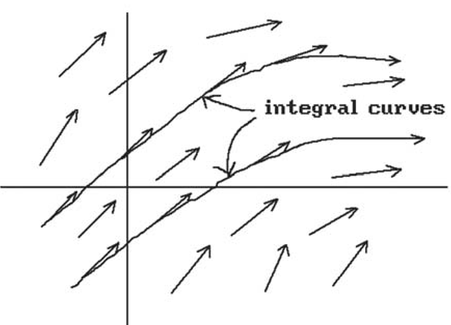
If y(x) is any solution, then f(x,y(x)) specifies the slope of the graph of y(x) at the point (x,y(x)). In other words, if one thinks of the function f as specifying a vector field over the entire plane (to (x,y) in the plane we associate the vector (1,f(x,y))), then solving equation (2.1) corresponds to finding a parameterized curvewhose tangent vectors agree with the vectors from this vector field. Mathematicians call such curves “integral curves.” In general, given a vector field, a curve whose tangent vectors agree with the vectors of that vector field at every point on the curve is called an integral curve for that vector field. See Figure 2.7. The reason for this nomenclature is that solving for the curve basically involves an integration process.

This idea of vector fields and integral curves leads to the following approach to finding numerical solutions to differential equations called Euler’s method. Suppose that we want the solution to pass throughSince    we know the tangent vector to the solution curve there and since the tangent line is a good approximation to the curve, moving a small distance along the tangent, say by where e is a small positive constant, will put us at a point _which hope fully is not too far away from an actual point on the curve. Next, starting at p1 we repeat this process. In general, let

Figure 2.7. Integral curves of a vector field.

Figure 2.8. Generating an integral curve approximation.

The sequence of pointsobtained    in    this    way becomes our approximation to the actual integral curve passing through p0.

Unfortunately, as we move from point to point we start drifting away from the actual curve and so our approximation will, in general, get further and further away from the true solution. To make the method work we need to compensate for any possible error as we move along. There are some very good algorithms that solve differential equations with basically this approach by using some fancy error-correcting terms. For more information see a text on numerical analysis such as [ConD72] or [DahB74].

Discrete curve-drawing algorithms that are based on the qualitative solutions to differential equations as described above are called digital differential analyzer or DDA type algorithms. Let us see what we get in the special case of straight lines.

The differential equation for the straight line that passes through the points andis

whereis    any    positive real number. Specializing the approximation formula, equation (2.2), to this differential equation gives us a sequence of points pi defined by

In fact, the points pi we generate will actually fall on the line, so that we do not have to worry about compensating for any errors. Although this may seem like overkill in the case of continuous lines, it does motivate an approach to generating discrete lines that leads to an extremely efficient such algorithm (the Bresenham algorithm). Note that if qi is the point with integer coordinates that is gotten from pi by rounding each real coordinate of pi to its nearest integer, then the points qi define a discrete curve that is an approximation to the continuous one. The key to getting an efficient line-drawing algorithm is to be able to compute the qi efficiently.

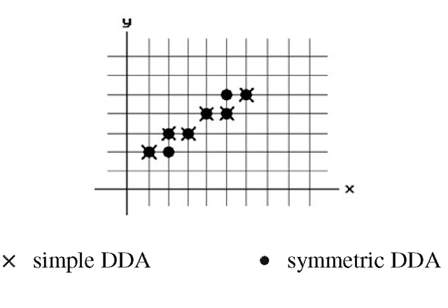
Figure 2.9. Simple and symmetric DDA generated lines.

In the continuous case one always generates points on the line no matter what e is chosen but the choice of e does matter when generating discrete lines. We now look at two possible choices for e. These give rise to what are called the simple and symmetric DDA, respectively.

 

Example. Suppose that we want to generate the discrete line from (1,2) to (6,5).

Solution. In this case

For the simple DDA we have

In the case of the symmetric DDA, we have

The points that are generated are shown in Figure 2.9. The points of the simple DDA are shown as x’s and those of the symmetric DDA are shown as solid circles.