Intersection Algorithms (Geometric Modeling) Part 3

Surface Sections

We begin our look at surface-surface intersections with the special case of finding a section of a surface S. This includes the problem of finding contours, although we will say more about that in Section 14.6.

Definition. The intersection of a set in Rn and a hyperplane is called a section of that set. If the hyperplane is parallel to a coordinate plane, that is, if it is defined by an equation of the formwhere c is constant, then the section is called a contour.

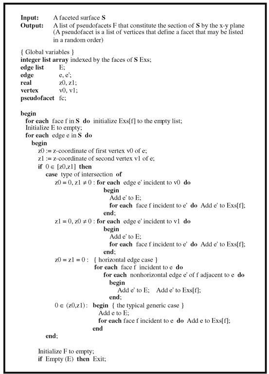
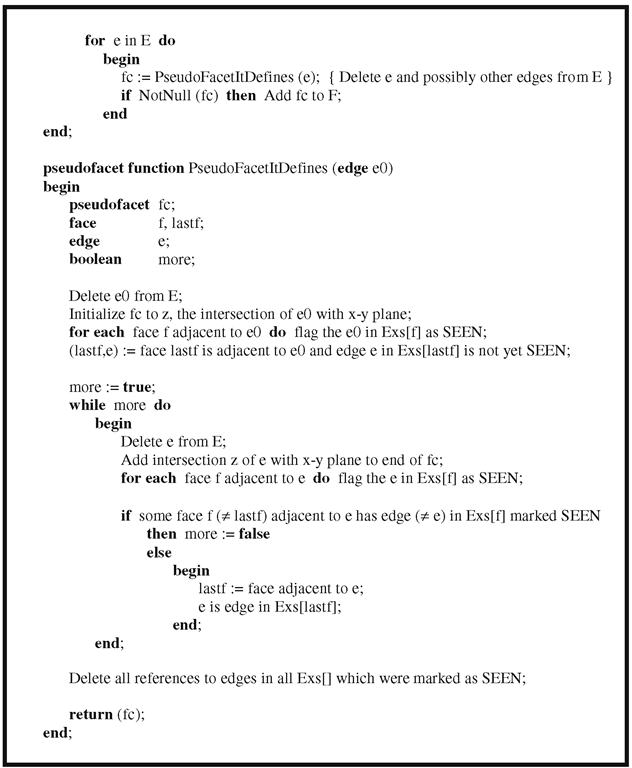
We first consider the case where S is faceted. Assume that S has convex facets. To find the section of S with respect to some plane there is again no loss of generality by assuming that the plane is the x-y plane. The idea will be to find all the edges of S that cross the x-y plane and then to connect the intersection points appropriately. To find the crossing edges, we only need to look at the z-coordinates of the endpoints of the edges and see if they straddle 0. To facilitate connecting the edge intersections we use the fact that if the section crosses a face then it crosses two of its edges (unless it just touches the face in an edge or vertex). Therefore, we associate a pair of integers to each face which will either both be -1 or the index of an edge in the edge array. The resulting algorithm is shown in Algorithm 13.4.3.1.

The problem of finding sections of smooth surfaces is more complicated. We have actually run into this problem earlier in the topic. In fact, some of the techniques described in Section 7.10 that provided a scan line visible surface determination algorithm for smooth surfaces would also apply to solve this problem. Here we describe another approach. See [PraG86] or [Sutc80].

The Grid or Lattice Evaluation Method. First of all, we may again transform the intersection problem by a rigid motion to the case where the plane is parallel or in fact equal to the x-y plane. The problem then is equivalent to finding a contour on a surface. If the surface is parameterized by a function

then the problem is to solve the equationThe basic idea is to reduce the problem to a lower-dimensional one by adding some constraints. Typically, one evaluates z(u,v) at a grid of pointsLetIf adjacenthave opposite

signs, then the contour will cross the corresponding edge between the grid points. One finds the crossing point by solving a one-dimensional problem of the form

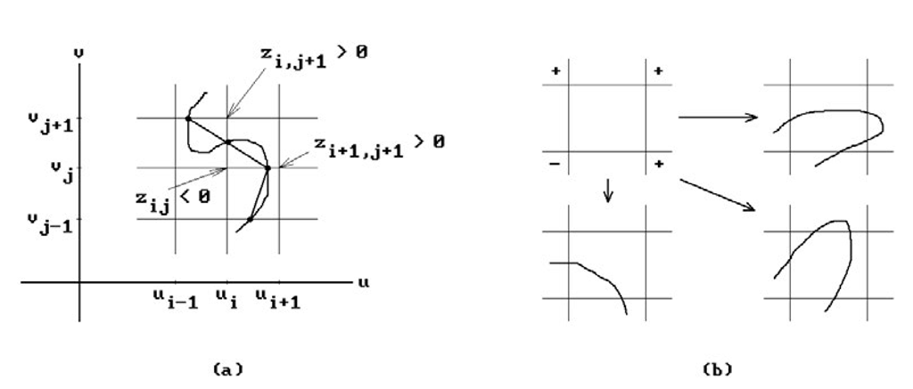
The intersection points are then connected to get a polygonal approximation of the contour. See Figure 13.9(a). One major problem with this approach is that it can be difficult to determine how to connect intersection points on the grid lines.

Figure 13.9. Sections using a lattice evaluation method and ambiguities.

Algorithm 13.4.3.1. A faceted surface sectioning algorithm.

Algorithm 13.4.3.1. A faceted surface sectioning algorithm.

A second problem is that some loops may be missed entirely if the grid is not fine enough. This problem often occurs near critical points of z(u,v), such as saddle points, or other singularities because the data may not have a unique interpretation. In Figure 13.9(b) there are three possible intersection curves that give rise to the same labeling of grid vertices with the sign of their z;j values.

[Faro87] describes an algebraic geometry approach to finding sections of bicubic patches. See also [ChaK87]. Another surface section algorithm is a special case of the general surface intersection algorithm described in [GraK97].

The problem of finding sections has a converse, namely to describe a surface given a collection of sections for it. This is skinning problem and will be discussed in Section 14.7.

Surface-Surface Intersections

General surface intersection algorithms are particularly important in geometric modeling, such as in the boundary evaluation algorithm of CSG and NC cutter path generation. Unfortunately, finding such intersections is a very difficult problem and no algorithm that is both efficient and correct is known at the moment. Efficient algorithms have problems near singularities or almost-singularities because computers only have finite precision. Accurate and robust algorithms are currently too slow. Some are based on algebraic geometry methods that do not apply to nonalgebraic surfaces. Others try to use interval arithmetic ([HMPY97]). Pratt and Geisow ([PraG86]) give a good survey of some older known intersection algorithms. [Fari92b] contains a list of references on the topic of intersection algorithms.

First of all, finding the intersection of two faceted surfaces reduces to finding the intersection of two facets in 3-space. This in turn reduces to finding the intersection of a convex polygon with a plane and then finding the intersection of a segment with a convex polygon. The mathematics behind doing this was discussed in Section 6.5. If only one of the surfaces is faceted and the other is smooth, one can reduce this problem to finding sections of the smooth surface and finding the intersection of two curves in these sections. This leaves the problem of finding the intersection of two smooth surfaces.

Like in the curve case, one approach to finding intersections of smooth surfaces that one might think of almost immediately is to approximate them by faceted surfaces and then use methods for intersecting those types of surfaces. The usual problem is deciding when an approximation is good enough. [Grif75] and [Grif78] used this approach to display parametric surfaces. [HaAG83] starts off with coarse faceted approximations whose intersecting facets are then subdivided further appropriately. [RosR86] used meshes of isoparametric curves. [Turn88] used a two-surface bounding volume that generalized his curve intersection approach described earlier in Section 13.3.2. After finding points close to the intersection, a Newton-Raphson method was used to actually find points on it.

Rather than solving the smooth surface intersection problem by reducing it to the faceted case it is better to deal with it directly. The special case of quadric surface intersections has been studied extensively. See, for example, [FaNO89] and [Pieg92] and the references in those papers. The solutions to the general problem involve five basic approaches referred to as lattice evaluation methods, marching methods, homotopy methods, recursive subdivision methods, and methods based on algebraic geometry. When the actual complete surface intersection algorithms that have been proposed are classified as belonging to one of these approaches one must keep in mind that the algorithms usually consist of several stages and different methods can be used for the separate stages. Therefore, many algorithms are really hybrids that do not fit under any single roof as, for example, the ones described in [BarK90], [Kopa91], and [GraK97]. The next five sections will discuss the various approaches.

[MarM91] describes a parameterization for the intersection curve. [GarW89] represents the intersection curve algebraically, basically as an algebraic curve and a birational map between the plane and space curve. Bounding boxes are sometimes used in intersection algorithms and [FiMM86] gives some general bounds for surfaces.

Parallelism has also been used to speed up intersection algorithms. See [BurS93] and [ChBA94].

Surface Lattice Evaluation Methods

A common special case of the lattice evaluation method was already described in Section 13.4.3 in the context of finding contours of the graph of a function of two variables. For more general surface intersection algorithms the method is used at most as a preprocessing step to get some starting points in the intersection. Given two parametric surfaces p(u,v) and q(u,v), one considers the lattice of curves p(ui,v) and p(u,vj) defined over grid lines in the rectangular domain of p(u,v) and finds their intersection with the surface q(u,v). The intersections give us starting points to which a marching method can be applied to find the complete intersection of the two surfaces. One might have to refine the lattice at places to make sure that no part of the intersection is missed. We shall see an example of this in the discussion of Timmer’s algorithm in the next section. In [BFJP87] polygonal approximations of the curves p(ui,v) and p(u,vj) were intersected with a polygonal approximation of q(u,v) and a Newton-Raphson method was then used to find real points on the intersection curves.

Surface Marching Methods

Marching methods, also sometimes referred to as tracing methods, are the most widely used methods for computing intersections. They assume that one has found points on the intersection and one then “marches” out from those points along the intersection curve by using information about the local geometry. We have already seen examples of this approach in other contexts. In general, this type of approach has three phases: a hunting phase, a tracing phase, and a sorting phase. In the initial hunting phase one tries to find start values that one then uses in the tracing phase to generate sequences of points that lie on the intersection. One needs enough start values, so that no part of the intersection is missed. Finally, in the sorting phase one separates the sequences of points generated by the tracing phase into sequences that define the connected pieces and loops that are the subcurves of the entire intersection. We end up with a discrete approximation to the intersection.

Figure 13.10. Hunting grids for Timmer’s algorithm.

An early marching method is one due to Timmer. See [Timm77] or [Mort85]. Suppose that two surfaces S1 and S2 have parameterizations p(u,v) and q(u,v), respectively, each with a rectangular domain. To find their intersection X, we shall find the subset of the domain of p(u,v) which parameterizes this set. The three solid curves in Figure 13.10 are an example of a set of parameter values for one possible such X.

Timmer’s Hunting Phase. Subdivide the domain of p into subrectangles. Restricting p to the associated grid lines defines a grid of curves p(u;,v) and p(u,vj) on S1. The intersections of these curves with S2 will provide the starting points that are used to trace the pieces of X. We run into the usual problem of making our grid fine enough, so that we will not miss any part of X. In Figure 13.10 the intersection of the grid lines with this set consists of points that have been numbered from 1 to 15. Let uv; denote the parameter point numbered i. The numbering is based on an ordering of the grid lines and the intersections that lie on them. We started with the vertical grid lines ordered from left to right and ordered their intersections based on increasing v value and then moved on to the horizontal lines ordered from bottom to top and ordered their intersections based on increasing u value. Actually, we do not really have to compute the intersection points precisely initially. They only need to be accurate enough so that a Newton-Raphson method, say, can be used to converge to the actual values. Therefore, the initial guesses for the intersection points could be found by discretizing the curves p(u;,v) and p(u,vj) also. Alternatively, we can think of the problem as one of finding points on a curve that are closest to a surface and use any algorithm that is known to solve this problem. Once we have our intersection parameter values uvi we start the next phase.

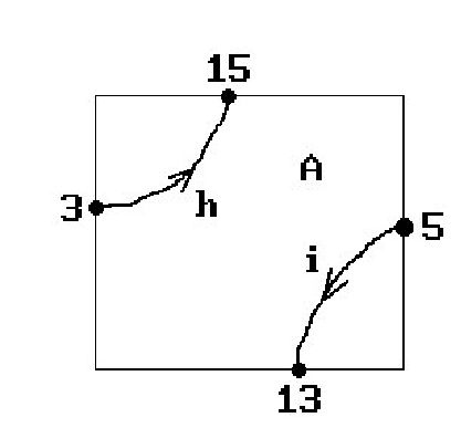
Timmer’s Tracing Phase. We consider the part of the intersection over each subgrid separately. We analyze each subgrid one after another based on a left to right, bottom to top order. Figure 13.11 shows the subgrid labeled A in Figure 13.10. Since the points uvi correspond to endpoints of curves in the subgrid, we now use them one at a time based on their ordering to trace the parts of the curves that lie in the subgrid. This not only gives an ordering to the pieces but also a direction. Figure 13.10 also showed the ordering, indicated with the labels a, b, . . ., k, and the direction in which curve segments were traced.

Figure 13.11. Curves in a hunting subgrid.

Figure 13.12. Determining the step size in Timmer’s algorithm.

The actual tracing of the curves is carried out using a standard Newton-Raphson approach, but it is worth commenting on how two details were implemented.

First, tangent vectors for the curves were used for stepping. They are obtained from the normals to the surfaces provided that the surfaces are not tangent at the point of intersection. Specifically, ifis    a    point    in    the    intersection X, then

is a tangent vector to X at x. Note however that we are making all of our computations relative to p(u,v), so that we have the parameterbut not.    To get the parametersanother    iterative procedure is used that, given a point x, solves an equation of the type

for (u,v).

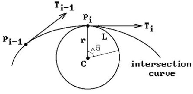
Second, one needed to decide on a step size L. See Figure 13.12. Suppose that we are at point pi. Let Ti be the unit tangent vector at pi. Let be the curvature of the curve at pi. This value can be computed using the first and second partials of p(u,v) and q(u,v). Let ri be the radius of curvature, namely, the radius of the osculating circle. Then ri is just the reciprocal of the absolute value of ki. The step size L is then defined to be the length riD0 of the arc from pi to A of the osculating circle with center C, where ΔΘ is some predefined constant angle tolerance. (It should be noted, however, that there is no need to actually compute the osculating circle because we only need the radius.) The pointin Figure 13.12 was then used as a starting guess for a Newton-Raphson iteration to get the next point pi+1.

Timmer’s Ordering Phase. We have to take our list of curve segments and combine them appropriately to get the complete curve. This is not totally trivial. Only the endpoints of the curve pieces are important. Basically, one starts with the first point uv1 and the piece to which it belongs, then looks for another piece that has an endpoint that matches the second endpoint of our piece, and continues in this manner. For the example in Figure 13.10 we would get following connected pieces:

This concludes our sketch of Timmer’s algorithm. The problem with Timmer’s algorithm is that it does not always give the correct answer and it is not as efficient as some more recent algorithms. Although more recent algorithms also fail at times, they give the correct answers in many more cases. We shall describe one more marching algorithm, namely, the one by Barnhill and Kersey ([BarK90]), although strictly speaking this algorithm is a hybrid method since it includes elements of recursive subdivision. Its primary goal was to be more general and more robust than previous such algorithms while still being efficient.

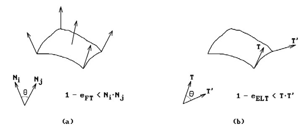
The Barnhill-Kersey Hunting Phase. The first step is to subdivide the rectangular or triangular domain of each of the parameterizations in an adaptive way. A quadtree data structure is used to represent a subdivision. Several types of subdivisions are performed. First, there is a uniform subdivision of the domain down to a user specified level for the quadtree. Then may come a further subdivision of those subpatches that do not meet a flatness and edge linearity criterion based on the angles between normals and tangents, respectively. For each subpatch we want the normals at the vertices and at one interior point to be almost parallel. Equivalently, the angles between them should be small. See Figure 13.13(a). In addition, for each edge of the subpatch, if T and T’ are the unit tangent vectors at the endpoints of that edge, then we also want those two vectors to be almost parallel or the angle between them small. See Figure 13.13(b). The eFT and eELT in the figures represent some predefined flatness and edge linearity tolerances, respectively.

Figure 13.13. Flatness and edge linearity tests in the Barnhill-Kersey algorithm.

At this stage, a parallelopiped bounding box is associated to each subpatch. Care must be taken in the definition of these bounding boxes so that they satisfy their essential property, which is that they contain their subpatch. The initial guess for a bounding box is determined from the vertices of the patch but is then enlarged using geometric information about the edge tangents and normal vectors. The subdivision is assumed to be fine enough so that the simple geometric argument that is used works. One uses the bounding boxes to cull away subpatches from the two surfaces that cannot possibly intersect. Determining whether two parallelopipeds intersect is done by transforming the second into the skew coordinate system determined by the first. The problem reduces to determining whether a parallelopiped intersects the unit cube and this has a straightforward solution.

Once one has found potential subpatch intersections, there may be some more subdivisions of those to increase accuracy and/or achieve convergence for subsequent Newton-Raphson steps. Suppose now that we have two bounding boxes that intersect, one from each surface. One then takes the average of the corner vertices of the subpatches associated to the bounding boxes and relaxes it to the intersection. One does this for every pair of intersecting bounding boxes. This will give us a collection of points on the intersection that are used as start points for the tracing stage, but before we get to that we want to describe how points are relaxed in [BarK90]. Such an operation is performed repeatedly in the tracing stage.

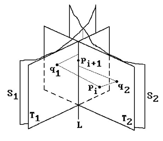
Relaxing Points in the Barnhill-Kersey Algorithm. Let p be the point to be relaxed. The point q in the intersection to which p is relaxed will be the limit of a sequence of points pi, where p0 = p. Assume that we have already found pi. We describe how the point pi+1 is defined. The first step is to find points q1 in S1 and q2 in S2 that are closest to pi. Ways to carry out this step are described in Section 14.2. If the points q1 and q2 are within a predefined same point tolerance eSPT, then we have found our q and we quit. Otherwise, let Tj be the tangent planes to Sj at qj. The point pi+1 will be the midpoint of the projections of q1 and q2 onto the line which is the intersection of T1 and T2. See Figure 13.14. Alternatively, let nj be a unit normal vector for plane Tj and define a third nonparallel plane T3 as the plane through the point (1/2)(q1 + q2) and normalThenis the intersection of the three planes and T3.

Figure 13.14. The Barnhill-Kersey relaxation algorithm.

The special case where the planes T1 and T2 are parallel is easily handled separately. Convergence, although a problem theoretically, was not a problem in practice given that points were only needed within the tolerance eSPT.

The method for relaxing points that we just described is what is used for determining the intersection in the interior of the surface patches, which is most of the time, but not for relaxing points onto the boundary of the patches. In that case one uses a Newton-Raphson approach to solve along with a parameter constraint determined by the boundary to which one is relaxing, for example, u = 0. We have a system of three equations in three unknowns. Parallel tangent planes are again a problem.

The Barnhill-Kersey Tracing Phase. This phase is started for each intersection point obtained in the hunting phase. For each start point, one generates a sequence of points that lie on the intersection. As one moves from one point p to the next one needs a step direction and step size. The tangent of the intersection curve at the current point is used as the step direction. Like in Timmer’s algorithm, this is computed from the cross-product of the normal vectors to the surfaces at p. One can save some multiplications by using Theorem 1.10.4(2) in [AgoM05] and use the direction

instead. Unfortunately, these formulas give the zero vector if the surfaces are tangent. In that case one can take the difference of previous intersection points. If there are no previous points and we are at the first intersection point, say

one samples points on the circles around (u0,v0) and (s0,t0) in the domains of the para-meterizations to find another point on the intersection. The new step direction is then taken to be the difference between this point and p.

Once one has the step direction one has to decide on a step size L. Like in Timmer’s algorithm one wants to use a formula of the formwhere r is the radius of curvature and ΔΘ is some predefined angle tolerance. However, the parameteriza-tions were only assumed to be C1 here and so the second derivatives are not directly available to compute this radius. Therefore, an approximation was used. Assume that we are a point p on the intersection. Two points a small distance e from p on the tangent line to the intersection curve at p are relaxed to points x and y on the intersection. The three points p, x, and y determine a circle and we let r be its radius because we can consider this circle to be an approximation to the osculating circle. Formula 6.8.1 implies that

where a = x – p and b = y – p. If the three points were collinear or L turned out to be larger than some predefined curve refinement tolerance eCRT, then L was set to ecRT·

Given a unit step vector v at a point p, we march to the next point p + Lv and relax it to the intersection. This describes the basic tracing step, but there is one more complication caused by what are called “terminating” points. These are points where the intersection curve

(1)    meets the initial point on the same curve segment, that is, the segment is a closed curve,

(2)    meets the patch boundary, or

(3)    meets an earlier curve segment.

Case (1) is simple and we indicated how case (2) is handled in the discussion of point relaxation. Points of type case (3) are discovered by checking for intersections of curve segments in the parameter space of the parameterizations. The points tend to be “branch" points, namely, places where multiple intersection curve segments meet. Once an intersection of parameter segments is found one has to find the branch point and make sure that the adjacent curve segments get sorted correctly.

Here is how one finds a branch point p. We take two endpoints pi and p2 of distinct crossing curve segments Ci and C2, respectively, as start points and then define a sequence of points pi. The points pi should alternate between lying on Ci and C2. See Figure 13.15(a). One continues generating pi until two successive ones are within a tolerance of espr* If there is no convergence, then we do not have a branch point. Here is how pi+i is defined, assuming that pi_i and pi have already been computed. See Figure 13.15(b). Let q be the orthogonal projection of pi on the tangent line to the intersection curve segment passing through pi_i. If ni is a normal vector to surface Si at pj_i, then

 

 

Figure 13.15. Finding branch points.

Figure 13.16. A branch convergence problem.

The point q is then relaxed to an intersection point that is defined to be p;+1. There are numerical problems if the tangents to the two curve segments at the branch point are almost parallel. A further problem is indicated in Figure 13.16. Suppose that we have detected an intersection in the parameter segments whose endpoints parameterize two pairs of points‘    .    In Figure 13.16(a), if we were to choose

p; and pj as start points of our iteration, then pj projects to the point A on the tangent line at p; and the point A relaxes to a point B which is again on the second curve segment. This violates our condition that our sequence of points should alternate between curve segments. If we had started with, say,as indicated in Figure 13.16(b), then everything would have been fine. To avoid this problem, Barnhill and Kersey suggest testing the angle between the vectorsIf

the angle is less than 90 degrees, that is,

then choose p; and pj, otherwise, choose p; and pj+1. There are numerical problems when the angle is near 0 or 90 degrees.

The algorithm in [GraK97] uses a different approach to finding terminating points in the case of tensor product spline surfaces. It uses an algebraic method for hunting and finds the terminating points before starting the tracing. The method is based on an algorithm that finds all solutions to the kind of nonlinear systems of equations one gets in the tensor product spline surface case.

Tolerances in the Barnhill-Kersey Algorithm. Several predefined tolerances were used in the algorithm. The main one was the same point tolerance eSPT. In [BarK90] it was claimed that assigning it a value of 10-7 gave good results on a computer with 16-decimal-place precision. It was also recommended to use tolerances based on angles as much as possible to remove dependencies on surface magnitudes and units of measure.

The Data Structures in the Barnhill-Kersey Algorithm. The main structure is that of a quadtree node. Each such node maintained the following information: its level, the coordinate transformation and its inverse for the associated bounding box, edge linearity and flatness measures, the parameter domain, the values, partials, and normals at the vertices and the centroid, a pointer to a doubly linked adjacency list used for sorting, and pointers to child nodes.

An adjacency list node consisted of a pointer to a doubly linked list of nodes that contained intersection information, namely, the start and endpoint of the domain of the segment in the form of four reals u1, v1, u2, and v2, the start and endpoint p1 and p2 of the segment in R3, and a flag indicating whether the segment terminated.

There was a list of pairs of quadtree nodes whose bounding boxes intersected.

The Barnhill-Kersey Sorting Phase. The quadtree data structure facilitated the sorting phase, but is not necessary. Note that all non-closed polygonal curve segments generated by the tracing phase terminate at boundary or branch points. When sorting those segments, endpoints are considered the same if they are within a tolerance of eSPT. The recursive divide-and-conquer algorithm described in [HEFS85] was used on the partial adjacency lists associated to the quadtree nodes.

This finishes our discussion of the algorithm in [BarK90]. The authors compared their algorithm to others, in particular to those in [BFJP87] and [HEFS85]. The advantages were that it also worked for parameterizations with triangular domains, did not need second derivatives, and handled more tricky cases correctly. It was at least as robust or more than other surface intersection algorithms. The tolerance constants described above could be adjusted manually to achieve better results in difficult cases. The reader might also look at the algorithm in [Luka89] for additional details on the Newton-Raphson mathematics.

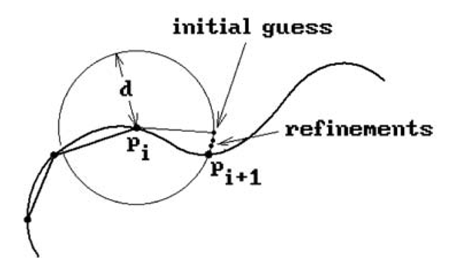
As a third example of a marching method for finding the intersection of two surfaces, assume that the intersection curve lies in the uv-plane, is defined by an equation f(u,v) = 0, and we have already computed the ith solution point p; = (u;,v;). Of course, one can look at this version of the intersection problem from various points of view. It can be thought of as an implicit curve or contour problem. Sections 14.5.1 and 14.6 discuss those. Here we shall describe a “step constraint” approach for getting the next point. Let us add another constraint g(u,v) = 0. For example,

corresponds to requiring that the next pointis on the intersection a distance d from pi. A step in the direction of the tangent of the curve atis used as an initial guess and then a Newton-Raphson method is used to converge to the next solution. See Figure 13.17. There are the usual potential problems such as needing a start point on the intersection curve and possible lack of convergence where the partials of f vanish.

Figure 13.17. A step constrained marching method.

Additionally, the step constraint must be chosen carefully. For example, for a constraint of the type shown in equation (13.15), the step size d influences the result and the value of d may change from point to point. We do not want to step to another branch of the curve. We also have to check for the possibility that our solution takes us outside the given (u,v)-domain. If the intersection curve is closed, then we also want to be able to close our curve explicitly.

A fourth marching method approach tries to minimize a function that vanishes on the set of interest. For example, if the intersection is defined by

and we use a step constraint

then we could try to minimize

See, for example, [Powe72] or [PraG86].

We mention one last marching type approach. Here one uses vector fields and differential equations, where intersection curves are solutions to the latter. See, for example, [PhiO84], [Chen89], [MarM89], or [KrPW92].

At the heart of the typical marching method is the Newton-Raphson method. One ends up with a discrete approximation to the solution. As one generates the points one always starts with a guess for the next point and then uses the Newton-Raphson method to successively refine that guess until we get a point that lies on the actual solution set with desired accuracy. Let us recapitulate some of the common problems marching methods have to contend with:

(1)    They need starting points.

(2)    The direction and step size has to be selected very carefully to avoid missing entire pieces of the intersection or accidentally stepping from one component to another.

(3)    They get tricky to implement near terminating points.

(4)    They have problems at singular points.

What differentiates the various marching algorithms is how these problems are addressed. We finish this section with a discussion of these points.

When it comes to picking start points, we have seen how the Timmer and Barnhill-Kersey algorithms do it. For more on the subject we refer the reader to [AbdY97]. That paper discusses two general methods for picking start points along with an analysis and comparison.

The question of step direction and size really has to do with finding a good approximation to the next point on the curve. Obviously, the better these guesses are, the faster the Newton-Raphson method converges to the solution. Most of the time, the guesses are based on linear approximations to the solution. For example, a starting guess for the next point is often chosen from the points along the tangent line at the current point of an intersection curve. This is often only a crude guess. A higher-order approximation to the solution set would lead to quicker convergence of the Newton-Raphson method. [Stoy92] suggests using a second-order approximation, that is, parabolas. In that way one was also able to control the deviation of the actual intersection curve from its polygonal approximation.

We shall sketch the mathematics involved in getting higher order approximations. The details can be found in [BHLH88] and [Hoff89]. Consider the implicit/implicit case where the two surfaces S1 and S2 in R3 are defined by equations

As usual our object is to define a sequence of points _so  that  the polygonal curve they define approximates the intersection of S1 and S2. We need to describe how we get the first point and then how we get from one point to the next.

Assume that we are given a pointthat    lies    on the intersection of S1 and S2 and we want to get the next pointAssume further that the gradientsand

are not zero and that the surfaces intersect transversally at p. If any of these conditions are not satisfied, the approach that will be described here will probably fail and an algebraic geometry approach would be appropriate if f and g are polynomials. The general assumption we make here is that the intersection of S1 and S2 can be defined by an analytic function of the form

defined in the neighborhood of the origin withWe use the first m terms of  this power series to approximateThe case m = 1 corresponds to the usual linear approximation and so of interest here is the casespecifically  when m = 2 or 3.

To accomplish the goal, we need to solve for the

LetConsider    the    Taylor expansion

for f around p. Assume thatSinceTherefore,

if one substitutes the series (13.18) into (13.19) all the coefficients of the resulting power series in t must vanish. Setting the coefficients ofto    zero gives m equations in 3m unknownsApplying the same argument to the function g that defines the surface S2 gives another m equations. This underdetermined system of equations can be solved. By adding some additional geometric constraints dealing with the curvature and moving triad associated to the space curve g(t), one can get a unique solution. The way that the additional constraints are chosen affects the parameterization g(t) of the intersection of the surfaces. [BHLH88] and [Hoff89] also discuss how to choose the step δ. One has to watch out that one does not get outside the radius of convergence of g(t). This is not easy, but one can give bounds for the maximum step size. In the case m = 3 these depend on the second and third derivative of γ.

Having gotten an approximation to the next point on the surface intersection, one performs a Newton-Raphson iteration consisting of pointsto find the point pi+1 that actually lies in that intersection with as much accuracy as desired. One point to note is that what we just did for R3 easily extends to computing the intersection of n – 1 hypersurfaces in Rn.

Using higher-order approximations to curves takes computation time, which is why many algorithms are satisfied with linear approximations and step in the tangent direction. However, one must also decide on the step size. Intuitively, it makes a lot of sense to base the decision on the osculating circle since it is the best circle approximation to the curve at the point. Both the Timmer and Barnhill-Kersey algorithms step in the tangent direction and use the radius of the osculating circle to determine a step size. Since everything is an approximation anyway, the only question is how accurately we should compute the osculating circle and its radius r. Computing second derivatives is usually not cheap. Timmer’s algorithm did compute r exactly. The Barnhill-Kersey algorithm used an approximation to the real r. Neither algorithm actually tried to compute the osculating circle and only needed its radius. The algorithms in [CheO88] and [Aste88], on the other hand, actually stepped along the circle. The first applied to parametric surfaces and the second to implicit surfaces. The approximation in [WuAn99] is better yet for parametrically defined surfaces. The authors define an approximation to the osculating circle that can be computed efficiently and step in its tangent direction (not along the tangent to the curve). The equation for their circle is based on the current and previously computed curve point and tangent. Let T; denote the tangent to the intersection curve at point p;. Let C be the point that is the intersection of the following three planesdescribed in point-normal form:

The point C is then assumed to be the center of the circle. The plane of the circle is assumed to have normal vectorSee Figure 13.18. Degenerate cases are handled in the paper. One can show that this circle converges to the actual osculating circle as pi approachedThe marching distance is again taken to bewhere is a predefined tolerance. It was found that this method leads to a robust marching algorithm that

Figure 13.18. An approximation to the osculating circle.

(1)    has the same complexity but better accuracy than using the tangent vector direction,

(2)    is simpler than using parabolic approximations to the curve but not quite as accurate, and

(3)    is as reliable as continuation methods but is more general.

This still leaves open the question as to whether one has chosen small enough steps so as to find all parts of the intersection curves. Therefore, the methods need an add-on for loop detection such as is described in [SedM88], [SeCK89], [Hohm91], and [MaLe98]. This also applies to finding the start points. Unfortunately, it is very hard to set tolerances correctly.

The problem of terminating points was encountered in our discussion of the Barnhill-Kersey algorithm where we had to make a special case out of finding those points and dealing with them. Finally, the problem with singular points is that the Newton-Raphson iteration method involves solving linear equations and the matrices for these equations usually have very bad condition numbers at the singular points, which means that one loses all accuracy. The iteration may not converge or may miss parts of the intersection curves.

[KrPP90] describes a hybrid algorithm that is basically a marching algorithm but uses algebraic methods to make sure that no part of the intersection is missed. It applies to the intersection of an algebraic and a rational parametric surface. The key point was being able to detect all the “significant” points on the intersection curve. Those are the boundary points, turning points (where the normal vector to the curve is parallel to the u- and v-axis), and singular points (where the first partials vanish).