A mathematical fractal is obtained by iterative application of the Hutchinson operator. A Hutchinson operator, w, takes an arbitrary object and arranges several transformed (usually reduced) copies of the object. In mathematical terms, application of the Hutchinson operator can be described by
where S is a nonempty bounded set in the embedding Euclidean space Rn, wi describes the process of the transformation (reduction and translation) of each copy, and denotes the union of the subsets created by each of the N transformations. Repeated iterative application of the Hutchinson operator,![]() , will, after an infinite number of iterations, lead to an attractor A:
, will, after an infinite number of iterations, lead to an attractor A:
FIGURE 10.2 Example of a Hutchinson operator that creates four copies of the original object (a line of unit length), reduced in size to one-third and arranged in the manner depicted.
The attractor A is invariant under the specific Hutchinson operator used for its creation [i.e., A = w( A)], and it is independent of the original set S. Let us examine one specific example for a Hutchinson operator. This example operator takes an initial set, for example, a line of unit length, and creates four copies, w1 through w4, each of length 1. w1 shifts its copy to the left, w4 shifts its copy to the right, and w2 and w3 shift and rotate the copy (Figure 10.2).
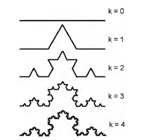
Repeated application of this specific Hutchinson operator creates a more and more jagged line (Figure 10.3). The attractor of this operation is called the Koch curve (named after Swedish mathematician Helge von Koch, who introduced this fractal object in 1904). It is interesting to observe that the Koch curve is infinitely long. The Hutchinson operator that generates the Koch curve arranges four copies of the original line (of unity length) that are reduced to one-third of its original size. The total length of the line at the first iteration, k = 1, is therefore At the kth iteration, the length is (3 )k, which goes toward infinity for k ^-<x>. Yet the curve is still bounded by the same length in both the horizontal and vertical directions. Furthermore, the Koch curve is self-similar; that is, any section of the curve, magnified, looks like the whole curve.
FIGURE 10.3 Iterative steps to generate a Koch curve.
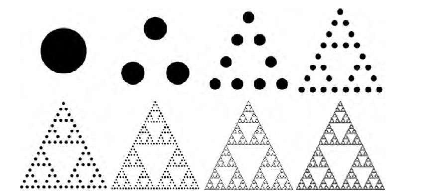
FIGURE 10.4 Iterative steps to construct the Sierpinsky gasket. The Hutchinson operator arranges three copies, which are reduced by a factor of 2, in a triangular pattern.
A different Hutchinson operator generates another well-known fractal, the Sierpinsky gasket. In this case, three copies, reduced by one-half, are arranged in a triangular pattern. Figure 10.4 shows eight iterations toward the Sierpinsky gasket. Notably, the attractor (the Sierpinsky gasket) is independent of the original set S, and in this example, the iteration starts with a circle as the initial bounded set S to demonstrate this property. If the original set has a total surface area of A, each of the reduced copies has a surface area of A/4 because of the factor-of-2 reduction of each side. Since three copies are arranged, the first iteration’s surface area is 3A/4. Analogous to the length of the Koch curve, the surface area changes by a factor of (4)k for the kth iteration. Evidently, the area occupied by the Sierpinsky gasket vanishes for k ^x. Although this fractal is embedded in a plane (the Euclidean two-dimensional space), one would intuitively not consider it a two-dimensional object because of its vanishing surface area. Yet it is not one-dimensional. A more rigid mathematical approach uses the scaling laws defined by the Hutchinson operator. In one-dimensional space, a reduction of a line by a factor of s allows us to place s scaled lines side by side within the same space. Similarly, in two-dimensional space, the reduction of a square by a scale factor of s allows us to place s2 of the reduced objects within the same area, and in three-dimensional space, s3 cubes can be placed within the same volume. The construction rule of the Sierpinsky gasket allows us to place a = 3 objects, scaled by s = 2, in the same space, and for the Koch curve, a = 4 objects, scaled by s = 1, may be placed in the same space. This relationship can be generalized with a power-law rule:
Here D coincides with the Euclidean dimensions 1, 2, and 3 for lines, squares, and cubes. For fractal objects, Equation (10.3) can be solved for D, and we arrive at the
where a is the number of copies arranged and s is the reduction factor. For the Koch curve (a = 4 and s = 3), the self-similarity dimension is D = log 4/log 3 « 1.26, whereas the Sierpinsky gasket (a = 3, s = |) has a self-similarity dimension of D = log 3/log 2 « 1.59. The dimensions are noninteger, leading to the term fractal. The noninteger dimensions of the two example fractals are intuitively acceptable. The Sierpinsky gasket, as identified before, is not really two-dimensional with its vanishing area. It is clearly not a one-dimensional object, though. With a dimension of approximately 1.59, it lies between Euclidean one- and two-dimensional objects. The same is valid for the Koch curve, with an infinitely long line folded in two-dimensional space. However, the Koch curve is more closely related (intuitively) to a line; hence its dimension is closer to 1, whereas the dimension of the Sierpinsky gasket is closer to 2.
Many natural objects have self-similar properties. The silhouette of a mountain range or the shoreline of a lake, even erosion patterns in volcanic rock, appear self-similar; that is, smaller sections, when enlarged, look like the whole. In nature, however, there is an aspect of randomness involved. Therefore, natural self-similar objects do not follow the strict rules applied for the construction of mathematical fractals. The inclusion of a random element in the Hutchinson operator is known to create naturelike shapes. In fact, artistic renderings of synthetic landscapes of strange beauty make use of random-based fractal generators (see, e.g., the comprehensive topic on procedural techniques by Ebert et al.,19 which makes extensive use of fractal methods). The principle of the process is demonstrated in Figure 10.5. The starting shape is a hexagon. For the first iteration, each of the six sides is split in two and the midpoint of each side is displaced by a random distance. At each iteration, the number of sides doubles. After a sufficiently large number of iterations, this process generates a shape resembling the coastline of an island. The key to creating a self-similar, fractal-like shape is the scaling element. The random numbers that determine the displacement must be multiplied (i.e., reduced) by a factor of 0.5kH at the kth definition of the self-similarity dimension D:
FIGURE 10.5 Iterative generation of the coastline of an island. The starting shape is a hexagon. From one iteration to the next, each side is split in two and the midpoint (the new vertex) is displaced a random distance. With each iteration, the coastline becomes more jagged and irregular.
FIGURE 10.6 Islands with coastlines generated by random walk to demonstrate the influence of the Hurst exponent H. With a small Hurst exponent, the coastline appears more jagged. A large Hurst exponent (close to 1) creates a relatively smooth curve.
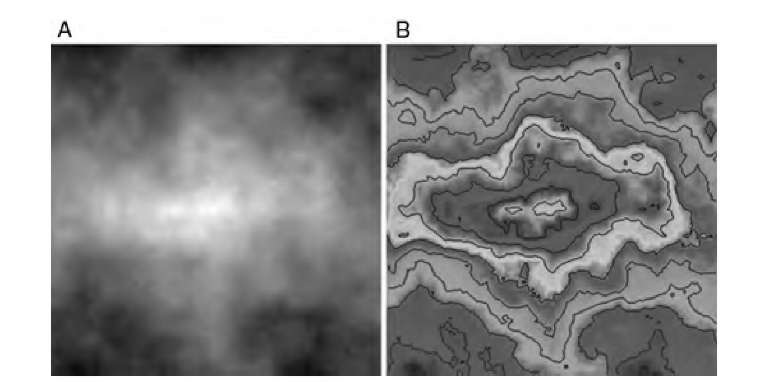
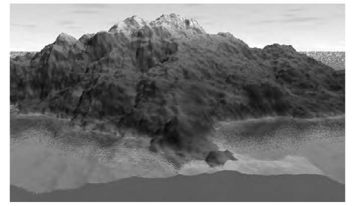
The same principle can be applied to obtaining three-dimensional landscapes. The starting object is a flat shape such as a rectangle. The rectangle is then subdivided into four triangles and each of the vertices is displaced by a random height. Each of the triangles is again subdivided, and each new vertex is displaced in height. This process is repeated iteratively several hundred times. A representative result of this process is shown in Figures 10.7 and 10.8. The displacement map can be represented in gray scale, resulting in a gray-scale image such as that shown in Figure 10.7A. A suitable false-color mapping combined with contour lines creates the topographical map in Figure 10.7B. Figure 10.8 is a three-dimensional rendering of the landscape with several added features: The landscape is colored based on the elevation, a sea level is defined (i.e., a threshold), and any gray value below the sea-level threshold is rendered as submerged; the water surface has received a mapped texture, and the sky is rendered with a mapped cloud texture.
FIGURE 10.7 Landscape generation using the iterative midpoint displacement technique. A shows the random displacements as gray values (light gray areas have a higher elevation than dark gray areas). With suitable false coloring and added contour lines, a topographical map is created (B).
FIGURE 10.8 Three-dimensional rendering of the topographical map shown in Figure 10.7, with elevation-dependent colors, texture-mapped sea level, and texture-mapped sky added.
These considerations pave the way for the analysis of medical images using fractal analysis tools. In a prominent example, the shape of lesions found in x-ray mammography images has been linked to their degree of malignancy.59,64 Irregular, particularly spicular, outlines indicate malignancy, whereas a more regular outline indicates a benign process (Figure 10.9). A strong relationship of the lesion outlines to the islands in Figure 10.6 is evident.
FIGURE 10.9 Abnormal masses in x-ray mammographies. (A) shows a circular, benign mass with regular outlines; (B) shows a spiculated mass with its irregular outlines. Irregular boundaries often indicate malignancy.
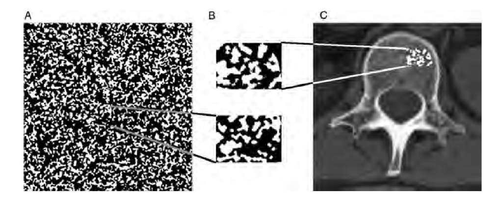
FIGURE 10.10 Similarity of the pattern of segmented trabecular bone (C) and a fractal generator that iteratively uses a neighborhood majority rule to set or reset a pixel (A). A small section of trabecular bone has been thresholded and magnified, and juxtaposed with an enlarged section of the fractal structure to demonstrate similarity (B).
A second image example for potential fractal properties are x-ray or CT images of trabecular bone. The fractal nature of trabecular bone has been subject to intense discussion (see e.g., references 12, 24, 42, and 48), but a number of studies that relate deterioration of trabecular bone to a change in fractal dimension are presented in Section 10.6. Let us consider an algorithmic process to create a fractal structure with a random element. On a square lattice filled with black pixels, white pixels are randomly seeded with a probability of about 50%. Next, we analyze each pixel and count the number of white pixels in a 3 x 3 neighborhood. If the majority of the pixels (i.e., five or more out of nine) are white, the central pixel will become white at the end of the analysis run. Otherwise (i.e., if the majority of the pixels is black), the central pixel will also be turned black. This run is now repeated iteratively until the pattern converges. A typical pattern that would result from this process is shown in Figure 10.10A. The pattern of segmented trabecular bone (Figure 10.10C) appears strikingly similar, as demonstrated in the magnified sections in Figure 10.10B.
Since natural objects with self-similar properties contain random elements, no construction rule exists to compute the fractal dimension analogous to the self-similarity dimension that we used on the Sierpinsky gasket and the Koch curve. It will therefore be necessary to investigate estimators of the fractal dimension, that is, numerical methods to assess self-similar properties in arbitrary images. The common principle of all estimators is to find the scaling rule (i.e., the power law) by taking iterative measurements at different scales. The principle can be demonstrated using the compass dimension. The length of a rugged outline is measured with different compass settings. As the compass settings become smaller, more detail is measured. A well-known example is the question of the length of the coastline of Great Britain.51 A compass can be used to determine the approximate, coastline length. In the example shown in Figure 10.11, a compass setting of 120 km leads to a polygon with 24 sides,corresponding to 2880 km.
FIGURE 10.11 Determining the length of the coastline of England with different compass settings.
With a 60-km compass setting, the compass can follow more details of the coast, and the new polygon has 56 sides and one incomplete side, corresponding to approximately 3390 km. In fact, with each smaller setting of the compass, more detail is captured, and the apparent length of the coastline increases. If we assume self-similar properties, we can expect the data pairs of compass setting s and measured length l to follow the power law described by
In Equation (10.5), D is the estimate of the fractal dimension. A similar power law was introduced in Equation (10.3). D can be determined by taking the logarithm of Equation (10.5) and thus obtaining the equation of a straight line that has the slope D and goes through the origin:
where lk and sk are the data pairs of compass setting s and the resulting length l for a number of different compass settings. D can now be determined by linear regression.
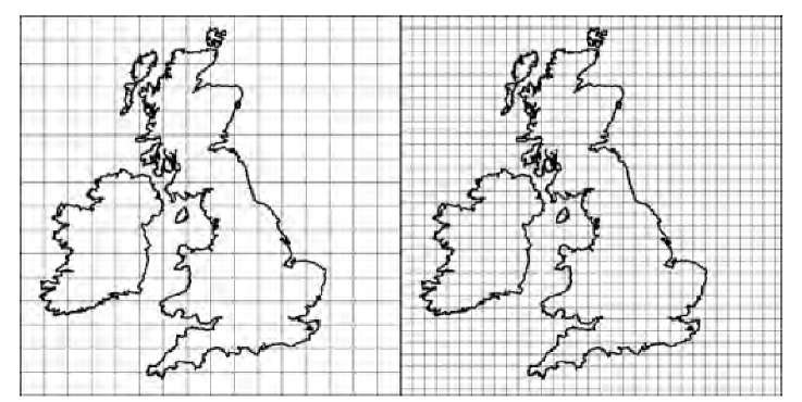
FIGURE 10.12 Determination of the box-counting dimension. The image is subdivided into squares of size s, and the number of squares that contain at least one pixel of the feature (in this case, the coast of England) is counted. Scaling properties are determined by repeating this process with different box sizes.


