Box-Counting Dimension
The box-counting algorithm is arguably the most widely used method to estimate the fractal dimension. The reason for its popularity lies in its simple computer implementation and its wide applicability to features with or without self-similarity. Furthermore, the box-counting algorithm can be carried out in two or three dimensions. To compute the box-counting dimension, the image is subdivided into equal-sized squares of side length s. Under the assumption of a binary image [background of value zero, image object(s) of nonzero value], all boxes that contain at least one nonzero pixel are counted. Then the box size s is increased by a certain factor, usually doubled (Figure 10.12). The resulting data pairs of box size sk and counted boxes nk are then log-transformed, and the box-counting dimension DB is determined by linear regression:
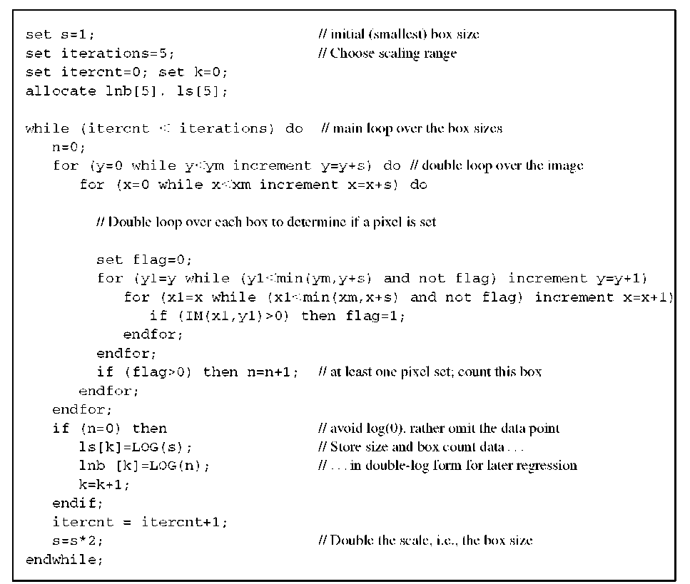
Pseudocode that performs a box-counting measurement as described above is provided in Algorithm 10.1. The algorithm expects a binary image and returns a table of box sizes log sk and corresponding box counts log nk. Linear regression into these data pairs yields the box-counting dimension DB . To provide a few examples, let us examine the Sierpinski gasket (Figure 10.4), with known exact self-similarity dimension, and the coastline (Figure 10.12), a random fractal with no known self-similarity dimension. Table 10.1 shows the box-counting results.
TABLE 10.1 Box-Counting Results for the Sierpinski Gasket and the Coastline
|
Box Size S |
Number of Boxes Counted |
Log (1/j) |
Log (Number of Boxes Counted) |
|||
|
Gasket |
Coastline |
Gasket |
|
Coastline |
||
|
1 |
26,244 |
12,336 |
0 |
4.419 |
4.091 |
|
|
2 |
8,748 |
5,922 |
-0.301 |
3.942 |
3.772 |
|
|
4 |
2,916 |
2,595 |
-0.602 |
3.465 |
3.414 |
|
|
8 |
972 |
1,132 |
-0.903 |
2.988 |
3.054 |
|
|
16 |
324 |
470 |
-1.204 |
2.511 |
2.672 |
|
|
32 |
108 |
193 |
-1.505 |
2.033 |
2.286 |
|
|
64 |
36 |
80 |
-1.806 |
1.556 |
1.903 |
|
|
Regression |
slope (= box-counting dimension DB) |
1.585 |
1.220 |
|||
|
r2 = |
1.000 |
r2 = 0.9991 |
||||
Algorithm 10.1 Box-counting dimension. The input image IM(x,y) is assumed to have the pixel dimensions xm and ym. A value of zero indicates a background pixel. The output are two corresponding tables of log box size ls() and log number of boxes Lnb(). The box-counting dimension DB is computed by linear regression and is the slope of the regression line into lnb over ls.
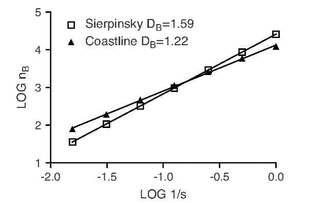
FIGURE 10.13 Graphical representation of the data in Table 10.1. The slope of the fitted data represents the box-counting dimension DB. In this example, the quality of the fit is extremely high, with r2 close to unity.
The graphical representation of the data in Table 10.1, shown in Figure 10.13, indicates a very good fit of a straight line in the log-log plot. It is crucial to verify the goodness of this fit, since several factors can affect the box-counting results. Most important, scaling limits exist: Box sizes smaller than the pixel size (theoretically possible through interpolation) will not yield reasonable results. At the other end of the scale, the data points will no longer fit the straight line either. If we superimpose four boxes over the Sierpinsky gasket (Figure 10.4), all four boxes will be counted. However, by merit of the construction rule, we know that the box count should be three. When the scale is reduced by a factor of 2 (a total of 16 boxes), 12 boxes would be counted where the construction rule allows for only 9. Only when the box size is much smaller than the object itself do the counts match the values predicted theoretically. The scaling rule fails in a manner similar to the coastline example. If we continue the box-counting process toward larger boxes, with the coastline as the object, a deviation can be observed as the data points follow a lower slope. A similar example is the fractal structure in Figure 10.10A. When the box size becomes larger than 8 (with a total image size of 512), all boxes are counted. For box sizes of 1, 2, 4, and 8, the resulting dimension is DB = 1.6, whereas a box-counting measurement that starts with a box size larger than 8 yields DB = 2.00, which is the Euclidean dimension of a plane. With unsuitably large box sizes, almost any value between 1.6 and 2 can be obtained.
In medical images, box counting at the pixel level will be confounded by the presence of noise. Gaussian noise contributes to the box-counting result on small scales. However, the r2 value of the linear regression may still be close to 1.00 and does not necessarily give an indication of a result confounded by noise. It is therefore important to examine closely at what scales self-similar properties can be expected and to select the box size range accordingly. Different modalities (e.g., a CT image and an x-ray image) of the same object may produce different dimension results, often as a result of different resolution. Even different exposure rates (e.g., x-ray images) may result in different values for DB. For this reason, many studies compare only groups with image acquisition parameters that are as consistent as possible.
The positioning of the box origins relative to the image features has a strong influence on the results as well. The example of the Sierpinsky gasket in Table 10.1 shows a perfect match with the self-similarity dimension only if the fractal object is aligned perfectly with the boxes. Shifting box origins relative to the features may produce biased values for DB that may be either too large or too small. The presence of multiple features (as in Figure 10.10A) may also lead to questionable results. Each feature may have its own self-similarity property, whereas the box-counting method yields only a single value. This value may not be characteristic for the structure analyzed. In this case it might be preferable to analyze each feature separately or to analyze the local scaling behavior and to examine the composition (histogram) of local dimensions of an image. This behavior is analyzed in more detail in Section 10.5.
Minkowsky Dimension
The Minkowsky dimension algorithm, also known as the capacitor dimension, uses morphological dilations to estimate scaling properties. The algorithm starts with the outline of the feature or image to be measured. Each pixel is then expanded into a filled circle of radius r, where r increases with each iteration. Some pixels of an expanded circle overlap with pixels belonging to neighboring circles. The total number of pixels gained (overlapping pixels are only counted once) is determined as a function of the dilation radius r, resulting in data pairs of np (the number of pixels) over r. The scaling law for the pixel gain is
where H is the Hurst exponent. In two-dimensional space, the fractal dimension D is related to the Hurst exponent H through
In the computer implementation, the initial feature outline is subjected to morphological dilation repeatedly and iteratively. For each dilation, the corresponding radius is identical to the iteration number (i.e., rk = k), and the pixels gained for iteration k, that is, np, k, can be determined by counting the total pixels of the original image, subtracted from the dilated image. For the data pairs rk and np, k obtained from several dilations, the Hurst exponent H and the fractal dimension D can now be determined by linear regression of the log-transformed data:
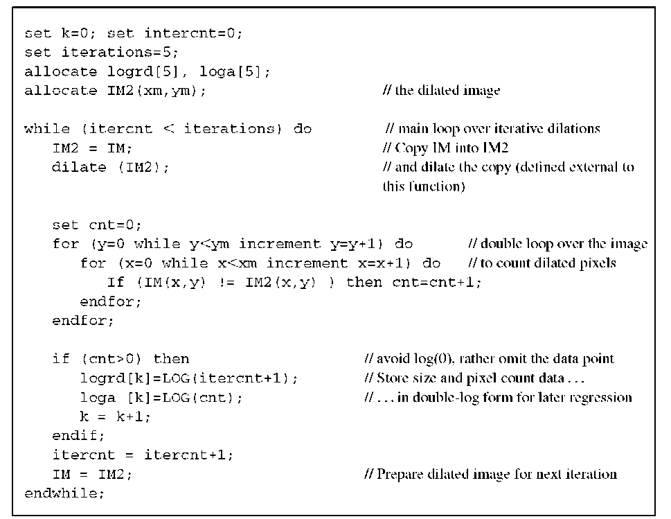
Pseudocode for a sample implementation of the Minkowsky dimension is shown in Algorithm 10.2. A few examples illustrate the process further. Individual dots, subjected to iterative dilations, expand to squares of 9, 25, 49,… total pixels. After one iteration (k = 2), the dilation operator has expanded the dots from 1 to 9 (by np = 8) pixels. This is the first data pair, (2,8). Subsequent iterations yield data pairs of (3,17), (4,32), (5,49), and so on. A linear fit into the log-transformed data yields a slope of H « 2 and therefore a dimension of D = 0, which coincides with the Euclidean dimension of the dot: namely, zero. A straight line would dilate into a "sausage" of thickness 2r. Its area would be approximately 2r l, where l is the length of the line. The area scales with an exponent of H = 1, giving the correct Euclidean dimension of 1 for the line. An example of a jagged line is presented in Figure 10.14. As an additional example, we apply the Minkowsky algorithm to the coastline of England (Figure 10.11). Over a large number of dilations, H = 0.74 is obtained, resulting in a Minkowsky dimension DM = 1.26. This value is in acceptable agreement with the dimension DB = 1.22 obtained through box counting.
The Minkowsky dimension method is less sensitive than the box-counting method to the placement of features. However, the Minkowsky dimension algorithm fails for filled two-dimensional shapes. Since the dilation process can only grow outward from the shape, the pixel gain is similar to the gain obtained with a one-dimensional shape (outline). In the coastline example, a dimension DM = 1.26 would be obtained irrespective of whether the shape of England is filled or the outline is used. Conversely, the box-counting method would yield a dimension of 1.83 for the filled shape as opposed to 1.22 for the outline.
Algorithm 10.2 Minkowsky dimension. Similar to the box-counting method, the input image IM(x,y) is assumed to have the pixel dimensions xm and ym. A value of zero indicates a background pixel. This function depends on morphological dilation, to be defined elsewhere. The output consists of two corresponding tables of log dilation radius logrd() and log dilated area loga(). The Minkowsky dimension DM is computed by linear regression. H is the slope of the regression line into loga over logrd, and DM = 2 — H.
FIGURE 10.14 Iterative dilation of a jagged line to determine the Minkowsky dimension. Shown are the original line (A) and the difference image after 10 (B) and 24 (C) dilations. It can be seen that a larger dilation radius causes filling of the jagged parts, so that the sensitivity to detail is diminished after several dilations. This property defines the ability of the method to determine scaling behavior.
Mass Dimension
The mass dimension, sometimes referred to as the sandbox dimension, is typically used on shapes with a clear center point, such as circular shapes or shapes with some level of rotational symmetry. Good examples are growth or aggregation processes that lead to dendritic structures growing out from an initial center point.21 Examples include neuronal patterns22 and structures found in melting carbohydrates.60 These structures bear a strong similarity to structures generated with a computer simulation, introduced by Witten and Sander.71 This type of simulated structure has been well explored, and it is known that they exhibit a fractal dimension of 1.7 over a wide scaling range with the mass dimension being the most suitable algorithm to use to estimate their fractal dimension.33,50,54 In fact, both the box-counting method and the Minkowsky method underestimate the dimension and yield values for D closer to 1.5.
Starting with this central point, the number of pixels of the feature inside a circle with radius r is determined. Then the radius is increased and the number of enclosed pixels is determined again. The result is a series of data pairs of counted pixels, np, as a function of the radius r. If the object underneath the expanding circle has self-similar properties, the number of pixels obeys a power-law scaling function:
In Equation (10.11), D is the mass dimension and is determined in a fashion identical to the box-counting method by log-transforming Equation (10.11) and fitting a regression line into the data pairs of log np and log r. The slope of this line is D.
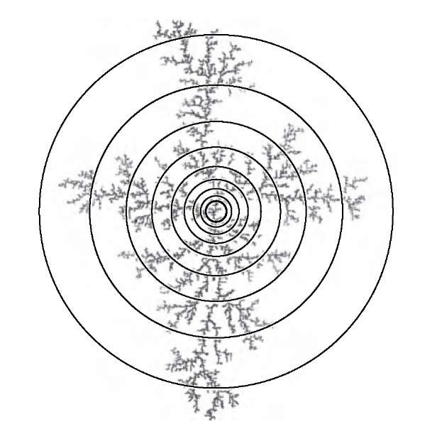
Figure 10.15 shows the use of circles of increasing radius to count enclosed particles. The corresponding plot of the particle count as a function of the circle radius is shown in Figure 10.16. Similar to all other fractal estimation methods, the mass dimension is sensitive to the choice of scales. As can be seen in Figure 10.16, the power-law relationship between particle count and circle size fails when the circle size reaches the aggregate size.
FIGURE 10.15 Determining the mass dimension of a simulated aggregation cluster. The mass (nonbackground pixels) of the aggregate inside the circles of increasing radius is counted, and the slope of the mass over the radius is determined on a double-logarithmic scale.
FIGURE 10.16 Number of particles enclosed in a circle plotted as a function of the circle diameter. This example shows the scaling limits particularly well. Whereas the particle count inside small circles (up to a radius of approximately 150 pixels) follows a power law with an exponent D of 1.74, the power law fails with large diameters once almost all of the aggregate is enclosed.
Unlike the Minkowsky method, the mass dimension is very sensitive against translations. A different choice of the circle’s center point may lead to highly different dimension values. At the same time, this property can be construed as an advantage, because it allows us to analyze a structure’s local properties. In fact, a mass dimension can be computed for each feature in a segmented image, or even for each pixel. In the second case, local fractal dimensions give rise to the concept of multifractals. These properties are examined more closely in Section 10.5.
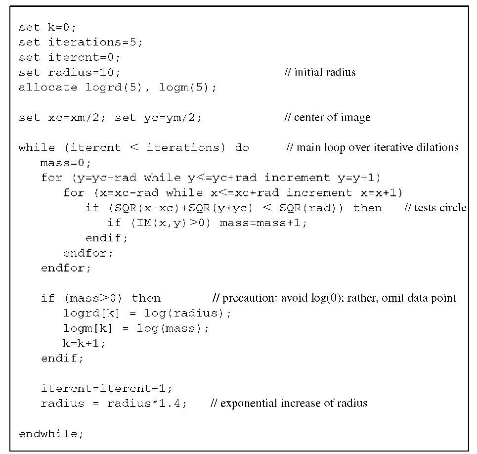
Algorithm 10.3 explains how the mass dimension is computed for a single feature in the image. Variations exist where square regions are examined instead of circular regions, and the radius step may either be exponential as in Algorithm 10.3 or linear. These variations will not provide fundamentally different results.
Algorithm 10.3 Mass dimension. Similar to the box-counting method, the input image IM(x,y) is assumed to have the pixel dimensions xm and ym. A value of zero indicates a background pixel. For the mass dimension, a suitable choice of the circle center (xc,yc) is crucial. In this example, the feature to be examined is assumed to be centered with respect to the whole image.

