Selected Topics for Further Research - Geomathematics: Theoretical Foundations, Applications and Future Developments - page 523

Box 12.6: Algorithm for Computation of Coefficients

In order to perform the required calculations it is convenient to

define an auxiliary function W j ( i , q )withasproperties W 1 i ðÞ ¼ ; q 0 ; W 0 i ðÞ ; q

p j q j W i q

N
j

¼ W i q ðÞ ¼ ðÞ k j i ðÞ ; q ð j ¼ 1, 2, ... N Þ . From the recurrence

formula for Krawtchouck polynomials, it can be derived that ( j +1) W j +1 ( i , q )
+[ i

Np + j ( p q )] W j ( i , q )+( N j +1) pqW j 1 ( i , of q ) ¼ 0. Consequently,

N N

the coefficients of ˈ 1 i ¼ ∑

j ¼ 1 c j k j ( i , q 1 )sa isfy c j ¼ ∑ j ¼1 ˈ 1 i W j ( i , q 1 ). The

correlation coefficient ˁ then can be obtained from the variance

1 c j 2

2 j W ( q 1 ) and, finally, the values

2 j

σ ¼ ∑ ˁ ˈ 2 i corresponding to ˈ 1 i become

¼

p 1
p 2

j ij

X N
j ¼0

p 1
p 2

i
j

ˈ 2 i ¼ 1 ˈ 1 j .

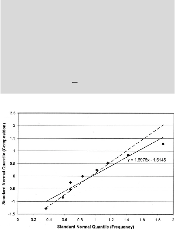
Fig. 12.52 Content of acidic volcanics in 768 square cells (Abitibi area, Canadian Shield)
measuring 10 km on a side; Q - Q plot of cell values similar to Fig. 12.46 (Source: Agterberg
2005 , Fig. 2)

For example, it will be attempted to determine the Abitibi acidic volcanics
frequency distribution of the 48 values for 40-km cells shown in Fig. 12.48 from
the frequency distribution of the 768 values for 10-km cells shown in Fig. 12.49
plus an estimate of variance s 2 ¼ 0.00386 for the 40-km cells. It can be assumed