Geoscience Reference
In-Depth Information
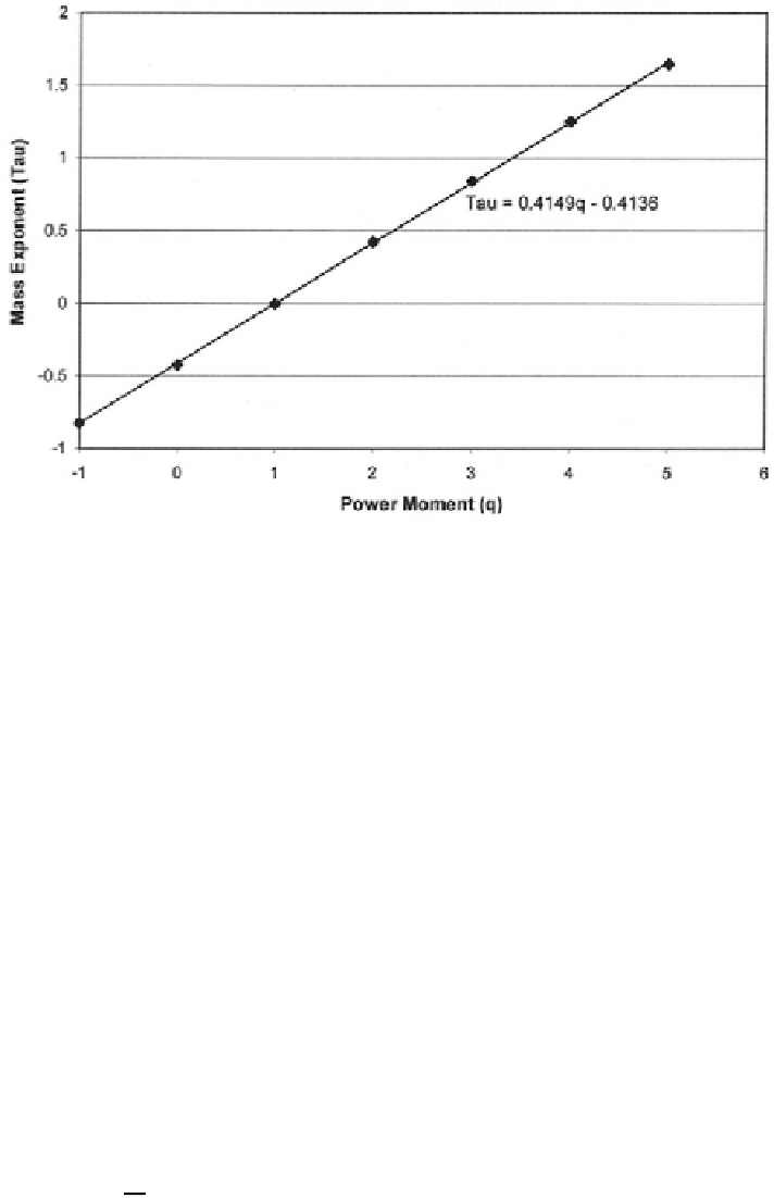
Fig. 12.51 Second step of multifractal analysis showing slopes of straight lines in Fig.
12.50
plotted against moment
q
. Result is a fractal with multifractal spectrum (not shown) reduced to
single spike for
f
(
ʱ
)at
ʱ
¼
0.41 (Source: Agterberg
2005
, Fig. 4)
12.8.5 Asymmetrical Bivariate Binomial Distribution
Matheron (
1980
) has suggested the use of discrete orthogonal polynomials of the
binomial distribution for empirical determination of the coefficients
c
j
and
c
j
*in
x
1
¼
ˈ
1
(
z
1
)
j
¼ 0
c
1
j
S
j
(
z
2
). Krawtchouck poly-
nomials can be used with, for example,
N
set equal to 10 or 20. An advantage
of this approach is that an arbitrary number of zeros can be accommodated
by choosing
q
N
N
¼
∑
j
¼0
c
j
Q
j
(
z
1
)and
x
2
¼
ˈ
2
(
z
2
)
¼
∑
nq
N
(
n
total
number of cells). Relative frequency of zeros decreases when cell size is
increased. With
N
remaining constant,
q
must decrease. An asymmetrical
binomial distribution can be used in which
z
2
is assigned a parameter
q
2
that
differs from that of
z
2
.Matheron(
1980
) has shown that setting
¼
1
p
for the binomial distribution do that
n
0
¼
¼
p
2
q
q
then
results in a suitable model. Using Krawtchouck polynomials
k
j
with squared norm
q
2
p
1
ˁ
¼
p
j
q
j
1
N
j
h
j
¼
j
¼0
c
j
k
j
(
z
1
)and
x
2
¼
ˈ
2
zðÞ
it follows that
x
1
¼
ˈ
1
(
z
1
)
¼
∑
j
k
j
zðÞ
X
N
j
¼0
c
j
q
2
q
1
¼
.

Search WWH ::

Custom Search