Chemistry Reference
In-Depth Information
1.00
1.00
0.98
0.98
0.96
0.96
10K 6T
0.94
11 K 8T
1.00
1.00
0.98
0.98
4K
0.96
10 K
0.96
-10
-5
0
5
10
-10
-5
0
5
10
V [mm/s]
V [mm/s]
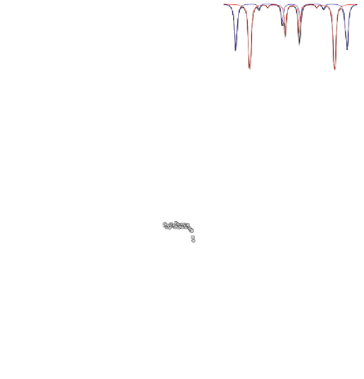
Fig. 4.6 Typical zero-field Mössbauer spectra (down) and in presence of an external field
applied parallel to the direction of c-beam on magnetite (left) and maghemite (right)
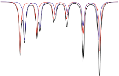
Fig. 4.7 Example of
Mössbauer spectrum recorded
at 300 K on as-prepared
assembly of magnetite
nanoparticles
1.00
0.98
0.96
0.94
n-Fe
3
O
4
300K
-10
-5
0
5
10
V [mm/s]
proportions; (2) the respective hyperfine field values can be estimated from Eq.
(
4.1
) and then (3) used to describe the zero-field Mössbauer spectrum. A dis-
agreement with experimental spectrum does give rise to think where it does come
from?
Several routes have been used to synthesize nanoparticles of magnetite: it is
usually observed for sizes below 40 nm, an increase of the intensity of the left
outer line giving rise to a change in the relative proportion of the two sextets as is
shown in Fig.
4.7
, and to a reduction of the mean value of the isomer shift. Then a
progressive collapse of the two sextets into a broadened and asymmetrical lines
sextet when the nanoparticles become much finer, preventing thus from an easy
modelling based on a discrete number of subcomponents.
The evolution of the relative proportions of the two sextets can be associated to the
progressive emergence of a component, the hyperfine characteristics of which are highly
close to those of maghemite. Finally, the 300 K Mössbauer spectrum allows to conclude