Graphics Reference
In-Depth Information
1.5
1
y
=
f
(
x
)
0.4
0.3
1
0
0.2
F
0.5
0.1
−1
0
−100
0
100
0
−
0.1
−
0.2
y
=
F
(
f
)(
)
20
−
0.5
−
0.5
0
0.5
−
20
0
20
0
S
B
−
20
1
0.4
−
0.5
0
0.5
0.3
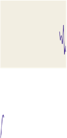
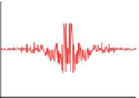
Figure
18.52:
A
non-band-
0.5
0.2
limited
function
and
its
F
−
1
0.1
transform.
0
0
−
0.1
−
0.2
−
0.5
−
0.5
0
0.5
−
40
−
20
0
20
40
Figure 18.53: To get from
ˆ
ftog, we multiply by a box B
(
ω
)=
b
(
34
)
; in other words, we
remove all high frequencies. To get from f to g, we convolve with the inverse transform of B,
namely a
sinc
of width
1
/
34
, that is, x
→
34 sinc
(
34
x
)
.
There's nothing special about the number 17 in this example. We can “band-
limit” the function
f
L
2
(
H
)
at any frequency
∈
ω
0
.
We can summarize the preceding two pages: If
f
is a function in
L
2
(
H
)
, then
to band-limit
f
at frequency
ω
0
we must convolve it with the function
x
→
S
(
x
)=
2
ω
0
sinc
(
2
ω
0
x
)
, or, correspondingly, multiply its Fourier transform by
)=
b
(
2
ω
0
)
. The result is the band-limited function
g
that's closest to
f
.
If you're thinking to yourself, “Gosh, computing the convolution involves an
integral, and doing that at every single point sounds
really
expensive,” you're right.
Fortunately, we'll never need to actually do this in practice.
ω →
B
(
ω
If you
did
want to approximate such a convolution, the practical method is
to take lots of samples of
f
, compute the “fast Fourier transform” (a discrete
version of the Fourier transform that runs in
O
(
n
log
n
)
time on
n
samples) on
these samples, remove all the frequencies greater than
ω
0
, and then transform
back again. That's how we made this chapter's figures.
As a second application, let's revisit what we saw in Figure 18.45: When we mul-
tiplied the Taj Mahal data by a “sampling” function, the Fourier transform began
to look periodic, as if it were made of multiple copies of the original transform,
overlaid and summed up.