Hardware Reference
In-Depth Information
154826.8
144826.8
134826.8
124826.8
114826.8
104826.8
Real
Feasible
94826.8
Unfeasible
Error
Virtual
84826.8
Feasible
Unfeasible
74826.8
Error
64826.8
Regression Line
54826.8
44826.8
34826.8
24826.8
14826.8
0
2000
4000
6000
8000
LOSS_value
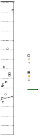
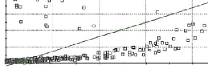
Fig. 7.13
Loss vs Mean Latency, from Node 1 to Node 0
As we can see in Fig.
7.10
, for a UDP application flow of 40 Mbps, the physical
flow is close to the application flow for low loss rates (with a small overhead). From
a loss rate of 20% on, we see that the transmission conditions start to degrade and
this is reflected in the fact that the physical throughput has to be increased in order to
cope with retransmissions of data. When the loss rate is bigger than 50%-60% even
the retransmissions and error corrections are not enough to keep the UDP throughput
and packets start to get lost.
In the opposite direction from Node 1 to Node 0 (Fig.
7.11
), since the application
throughput is very low (around 1 Mbps) the impact of data loss is reduced.
Figure
7.12
shows how the average latency obtained in the communication from
Node 0 to Node 1 is kept constant with low loss rates. When loss rate achieves a
significant value (35%), we start to see an increasing of the average latency making
the multimedia transmission impossible.
In the opposite direction from Node 1 to Node 0, Fig.
7.13
shows that the average
measured latency is kept almost constant for low loss rates, becoming a problem as
soon as the channel degrades. These results are similar to Fig.
7.12
.
As we can see, all the obtained figures are completely coherent with the expected
behavior of the system in real deployments based on previous generations of chipsets
and the theoretical analysis of the algorithms used. These figures can help us to
conclude some interesting data like the fact that the system can have a correct behavior
even under poor transmission conditions with a 40% of loss of packet. It is interesting


Search WWH ::

Custom Search