Information Technology Reference
In-Depth Information
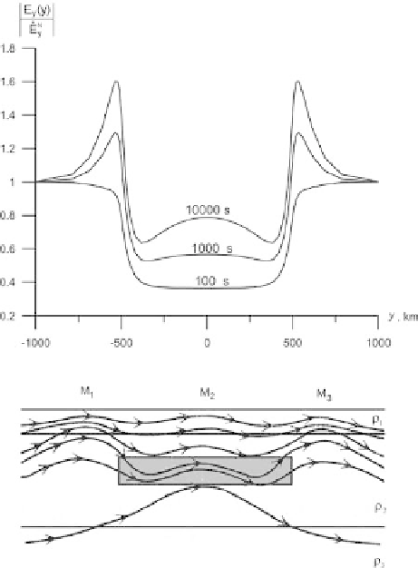
Fig. 8.4
Electric profiles
(TM-mode) passing across
the conductive zone shown in
Fig. 8.3. Model parameters:
1
=
·
,
h
1
=
,
10 Ohm
m
1km
2
=
2
=
·
,
1000 Ohm
m
h
2
=
19 km
,
h
2
=
15 km
c
=
10 Ohm
·
m
,v
=
500 km
,
2
=
500 Ohm
·
m
,
h
2
=
65 km
,
3
=
Profile
parameter: period
T
10 Ohm
·
m
.
=
100
,
1000
,
10000 s
with further lowering frequency when most of current is induced in the homo-
geneous
conductive mantle the magnetic anomaly almost completely decays
(
T
=
10000 s).
8.1.2 Magnetotelluric and Magnetovariational Response Functions
in the Model of Crustal Conductive Zone
Now examine the apparent-resistivity and impedance-phase curves observed in the
two-dimensional model from Fig. 8.3.
Figure 8.6 shows the transverse and longitudinal curves
⊥
,
⊥
and
,
together with the locally normal curves ˙
n
(over
the prism). They have been obtained at the different distances
y
from the epicentre
of the crustal conductive zone. The low-frequency branches of the transverse curves
⊥
,
⊥
observed over the central part of the prism are distorted (
y
n
,
n
(outside the prism) and ¨
˙
n
,
¨
=
0
÷
250km).
They are shifted down with respect to the locally normal curves ¨
n
. This gal-
vanic effect is accounted for by the transverse-current redistribution due to the
shunting action of the crustal conductive zone. Inasmuch as its intensity depends
on the prism conductance
S
c
=
n
,
¨
/
c
, it is termed the
deep S
-
effect
. Outside the
h