Information Technology Reference
In-Depth Information
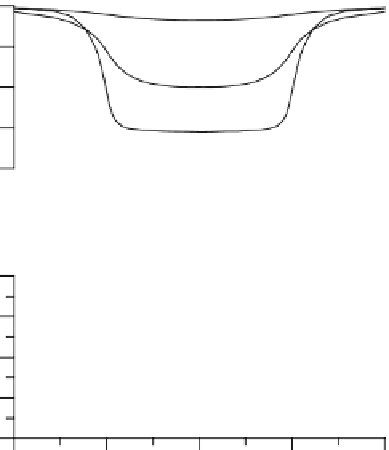
Fig. 8.5
Electromagnetic
profiles (TE-mode) passing
across the conductive zone
shown in Fig 8.3. Model
parameters:
1
=
1
10000 s
0.8
·
,
h
1
=
,
10 Ohm
m
1km
2
=
2
=
1000 Ohm
·
m
,
1000 s
0.6
h
2
=
19 km
,
h
2
=
15 km
,
c
=
10 Ohm
·
m
,v
=
500 km
,
100 s
0.4
2
h
2
=
500 Ohm
·
m
,
=
65 km
,
3
=
Profile
parameter: period
T
10 Ohm
·
m
.
0.2
y, km
-1000
-500
0
500
1000
=
100
,
1000
,
10000 s
100 s
100 s
1.2
1000 s
1.1
10000 s
10000 s
1
0.9
y, km
0.8
-1000
-500
0
500
1000
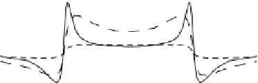
prism (
y
700 km) the deep
S
-effect shifts the low-frequency branches of the
transverse curves
=
501
÷
⊥
,
⊥
up. It quickly attenuates with distance and vanishes at
y
800 km. The formal one-dimensional inversion of the MT-curves distorted by
the deep
S
-effect yields a false elevation and false side depressions of the conductive
mantle.
Not so dramatic are the induction effects. The longitudinal curves
≥
,
are
essentially
distorted
only
near
the
edges
of
the
conductive
prism
- and
-curves with flattened descend-
(
y
=
499
÷
501 km). Here we observe the
ing branches. Away from the conductive prism (
y
=
600
,
700km) and over its central
,
merge with the locally normal
part (
y
=
0
÷
250 km) the longitudinal curves
curves
n
,
n
and allow for the one-dimensional inversion.
How does the dimension of the crustal conductive zone affect the apparent-
resistivity and impedance-phase curves? Figure 8.7 shows the apparent-resistivity
curves in the model where half-width
of the prism varies from 25 to 850 km. The
observation site is located at the epicentre of the crustal conductive zone (
y
v
=
0).
The conductive prism with
v
=
25 km is almost completely screened in the TM-
⊥
-curve shows no evidence of crustal conductor). But in the
mode (the bell-shaped
-curve, which has a gentle displaced minimum revealing the
presence of the conductive prism. Let us increase the prism half-width. In the case
v
=
TE-mode we see the
⊥
-curve has a small knee reflecting the crustal conductor, while the
-curve practically merges with the locally normal curve ¨
100 km, the
n
. The case
v
=
150 km
is of special interest. Here the prism half-width
v
is more than threefold adjustment