The 1500 Year Quasiperiodicity During the Holocene - Abrupt Climate Change: Mechanisms, Patterns, and Impacts - page 166

observed at the beginning of the nineteenth, twentieth, and
now the twenty-first centuries. Ogurtsov et al. [2005],
using the tree ring data, which is an Earth

(of about 0.1°C in the tropics) that increases the strength of
the Intertropical Convergence Zone (ITCZ) and shifts the
summer ITCZ to a more northerly position. The resulting
extra rainfall brings fresh water into the ocean lowering its
salinity. This salinity anomaly slowly propagates toward the
subpolar North Atlantic where it causes the AMOC

' is climate proxy,

have found a spectral band of 50 130 years. They divided

it into two components: one with 90 - 100 year period and
the second one having 50

-

60 year periods (see also Hath-
away [2010]). According to our model, it is the

- ow to

slow down to the weak state. In the weak state of the AMOC,
the ITCZ returns to its normal location thus closing the cycle,
which takes a century long period P c mostly de

rst
component of this proxy that beats with the centennial
ocean variability.
Coupled ocean-atmosphere modeling indicates that the
internal variability of the AMOC is well distinguished at
interannual and centennial time scales, with the centennial
(

ned by the
transport time of the salinity anomaly. Since this period of
natural ocean variability is close to the centennial Gleissberg
period P s = 90 years of solar variability, one may expect
beats between the two close periods: 1/P =1/P s

100 years) mode being dominant [Vellinga and Wu, 2004].
This mode, which is shown in Figure 4 of Vellinga and Wu,
also indicates an unstable, intermittent nature of this variabil-
ity. In the model this mode is excited due to the following
mechanism advocated by Vellinga and Wu: The AMOC in its
strong state produces a weak cross-equatorial SST contrast

≈ 1/P c . The

resulting modulation period would be equal to P = 1500
years for P c ≈ 97 years. Since, in reality, there is no strict

periodicity either in ocean or in solar variability, the beats are
expected to be unstable and thus in accord with observations,
suggestive of a nonlinear nature of oscillations.

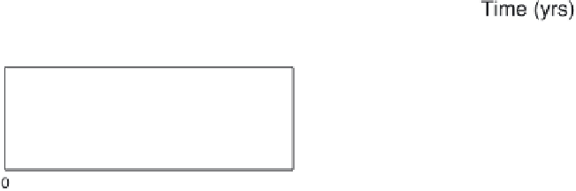
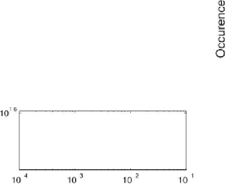
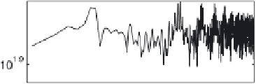
Figure 8. (left) A realization of the white noise forcing causes the system to randomly transit between two states marked
(middle) by 0 and 1. The resulting spectrum shows no speci

c features. (right) Aweak periodic forcing by two sinusoids
with close frequencies (1/90 year and 1/97 year), which simulate the solar and centennial ocean variabilities, groups the
transitions so that the beat frequency 1/1500 year is seen in the spectrum of the system response. The parameters used for
this realizations are p = 0.885 (to make the threshold equal to 1), a = 0.21, and b =1, = 0.1.

e