The 1500 Year Quasiperiodicity During the Holocene - Abrupt Climate Change: Mechanisms, Patterns, and Impacts - page 167

To convert the idea into a mathematical form, we consider
a simple conceptual model described by the equation

presenting the terms + p in equation (1) via a

potential ∂ / ∂ ϕ with U = cos ϕ + px having a potential
well corresponding to the stable state and unstable hump.
Equation (1) has been integrated in time using a stiff ODE
code from the MATLAB library. The value of e is chosen
such that the ocean and solar signal are smaller than the
threshold distance

sin

ϕ

d d t þ sin ϕ ¼ p þ a ⋅ N ð t Þþε ⋅ ½ O ð t Þþ b ⋅ S ð t Þ ;

ð1Þ

which is an extension of the equation introduced in the
context of stochastic resonance by Wiesenfeld et al. [1994].
Here p < 1 is a parameter which will define two basic states
of the AMOC (the weak and strong), N(t) is a random noise
of amplitude a, and e is a small amplitude of the ocean O(t)=
sin (2 π /P c ) centennial variability. The amplitude of the solar
signal S(t) = sin (2 π /P s ) is distinguished by an extra param-
eter b ≤ 1. The basic variable ϕ characterizes the state of the
AMOC, i.e., the magnitude of the flow.
Without the noise, ocean centennial variability, and solar
signal (N =0, e = 0), this system has two equilibrium states
defined by the condition sin ϕ = p: a stable ϕ s = a sin (p)
state and an unstable ϕ w = π a sin (p) state, which we can
associate with the strong and weak states discussed above in
the observational context. The stability of these states can
easily be checked by a perturbation of the equilibrium or by

2 arcsin (p) between the two states,
and thus these forcings alone cannot move the system from
one state to another. At

ϕ

= 0, driven only by the irregular

e

noise kicks, the state point jiggles around the stable strong

state and, from time to time when the amplitude of an event is
large enough, goes over the threshold and moves into the
unstable weak state. After about a mean residence time in the
unstable state, sec ( ϕ s ), the point returns back to the stable
state. The noise forcing alone produces a random sequence
of events. However, when

ϕ

0, the added ocean-solar
forcing produces different outputs via modulating (grouping)
the random transitions between the states so that the 1500
year signal arising from the beats becomes feasible. Figure 8
shows two specific examples of numerical solutions of equa-
tion (1): the

e ≠

first one with the white noise input only (left
plots) and the second one with the addition of the periodic

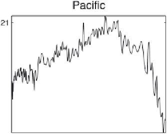
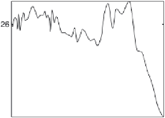
Figure 9. Reconstructed SSTs (top) for the Paci c Ocean at 62.05°N, 17.49°W [Isono et al., 2009] and (bottom) near the

Nile delta (10.70°N, 64.94°W at the depth 790 m) [Castañeda et al., 2010].