Biomedical Engineering Reference
In-Depth Information
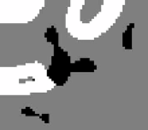
Figure 5.7:
Maximum a posteriori classification. Cross-section with the MAP
labels. Black corresponds to the vessel tissue, white to bone and gray to the
background.
This Partial Differential Equation verifies the Maximum Principle [25]. There-
fore, the posteriors remain being probability functions after diffusion. Applying
anisotropic diffusion introduces spatial coherence before the MAP decision thus
improving the classification results [26]. Figure 5.7 shows one example of the
MAP classification. Voxels labelled as vessel are used as initialization of the GAR
method introduced in the next section.
5.2.4
Geodesic Active Regions
5.2.4.1
Geodesic Active Contours
Caselles
et al.
proposed an implicit deformable model known in the literature as
Geodesic Active Contours [27]. It conciles Parametric Models and the Level Set
Theory. It is based on the idea from geodesic snakes [28] of evolving an initial
curve to a local minimum of an energy functional.
The GAC energy functional is defined for surfaces as
g
(
S
)
da
E
(
S
)
=
(5.7)
where
S
represents a parametrization of the evolving surface,
g
is an inverse
edge detector function, and
da
is the surface area element. This energy functional
defines a Riemannian Space, with metric associated to the edge detector function
g
. The geodesic surfaces on this space, are defined by the edges of the image.
To compute the differential equation that drives the evolution of the sur-
face, traditional variational techniques are used. The Euler-Lagrange equation