Biomedical Engineering Reference
In-Depth Information
(a)
(b)
(c)
(d)
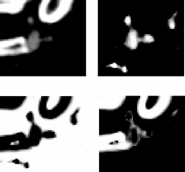
Figure 5.6: Cross-section of the PDF images estimated by the kNN rule. Brighter
areas correspond to higher probabilities. (a) Gray level image. (b-d) Probability
for vessel, background and bone, respectively.
belong to a certain class,
P
(
I
(
x
)
=
i
|
x
∈
C
j
). All tissue classes are assumed to
be equiprobable.
The Bayes rule is then applied to calculate the posterior probability for a given
voxel to belong to a particular class given its intensity,
P
(
C
j
=
c
j
|
I
(
x
)
=
i
).
The MAP classifier uses the maximum a posteriori probability estimate after
anisotropic smoothing [24] to obtain a classification of the voxels of the image
C
j
=
arg
max
c
j
∈{
C
0
,
C
1
,
C
2
}
P
∗
(
C
j
=
c
j
|
I
(
x
)
=
i
)
(5.5)
where
P
∗
corresponds to the posterior probabilities after diffusion driven by
the equation
∂
t
=
div
∇
P
1
/
3
∂
P
|∇
P
|
(5.6)
|∇
P
|