Geoscience Reference
In-Depth Information
2. For lesser values of
H
that lie within the multiple equi-
librium regime
H
c
£
H
£
H
c
, a finite perturbation that draws
A
below the unstable equilibrium
A
e
also will result in an
abrupt transition to
A
= 0. Conversely, a sufficiently large
positive perturbation from
A
e
will induce a transition to
A
+
.
Hence, in this regime, sufficiently large fluctuations can re-
sult in “switching” between the two stable equilibria, a phe-
nomenon examined further in section 3.4.2.
3. As
H
increases toward
H
c
, the impact on
A
of fluctua-
tions in
H
steadily increases. This tendency can be quantified
by considering the sensitivity of
A
to changes in
H
. If (
T
n
,
A
n
) initially are in equilibrium on the upper stable branch at
some
H
<
H
c
, then the response of the following year's sum-
mer sea ice extent to an incremental OHT increase
dH
is
A
should occur in the neighborhood of abrupt transitions as
appears to be the case in Figures 1 and 7. This phenomenon
and the potential for its observational detection are discussed
further in section 3.5.
The dependence of the equilibrium solution structure on
the parameters in (6) - (8) is now considered, as this may
bear on the widely differing responses of Arctic sea ice to
climatic warming among different climate models, which
is discussed briefly by HBT, as well as the model inter-
comparisons of
Flato and Participating CMIP Modelling
Groups
[2004],
Arzel et al.
[2006], and
Zhang and Walsh
[2006].
3.3.1. Dependence on F and b.
A key feature of the equi-
librium solutions to (6) - (8) with parameter values fit to
CCSM3 behavior as described above is the multiple equilib-
rium regime that occurs for
H
c
<
H
<
H
c
and the attendant
hysteretic transitions, as illustrated in Figure 9. The transi-
tion relevant to a warming climate is the one from
A
e
to
A
e
that occurs as
H
increases through
H
c
. Two key parameters
characterizing this transition are the critical ocean heat trans-
port
H
c
, given by (A3), and the minimum stable sea ice area
A
e
(
H
c
), which determines the magnitude of the transition.
Figure 11 illustrates the dependence of these quantities on
the baseline ice formation parameter
F
and ocean shortwave
absorption parameter
b
, with remaining parameters fixed at
CCSM3 values. (The strength of ice-albedo feedback may
be sensitive to the type of ice model employed, for exam-
ple multiple versus single thickness category [
Holland et
al.
, 2006b], whereas winter ice thickness is known to dif-
fer widely among climate models [
Flato and Participating
CMIP Modelling Groups
, 2004]). The CCSM3 values for
F
and
b
are indicated by the asterisk, and letters a - d sig-
A
n
+1
−
A
e
(
H
)
dH
dA
dH
|
A
e
(
H
)
º lim
|
|
dH
®0
é
ê
ë
M
(
s
0
+
M
(
b
0
+ (
T
e
+
wH
)(1 +
A
e
/
A
max
)/ 2
1
+
(
T
*
/
T
e
)
wH
/
2
= -
A
max
T
*
w
T
e
,
2
H
<
H
c
,
(11)
where
T
+
(
H
) and
A
+
(
H
) are given by (A1), (A2), and (A4).
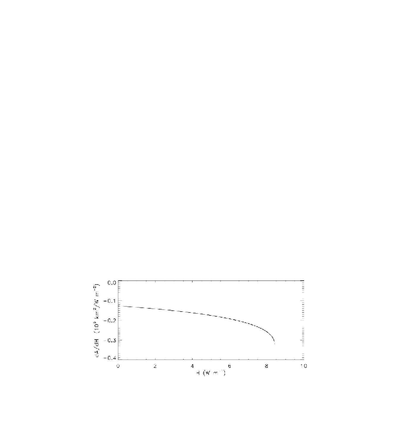
This sensitivity, plotted as a function of
H
in Figure 10, be-
comes increasingly negative as
H
approaches
H
c
, implying
that sensitivity to fluctuations in
H
amplifies as the hyster-
etic transition is approached. This result, together with the
tendency for OHT fluctuations to increase as
H
increases
(Figure 4b), suggests that particularly large fluctuations in
Figure 10.
Sensitivity
dA
/
dH
of summer ice extent
A
to fluctuations in
H
when the system is perturbed from equilibrium
on the upper stable branch
A
e
for the case illustrated in Figure 9.


Search WWH ::

Custom Search