Environmental Engineering Reference
In-Depth Information
With this defined properties, a finite element
method (FeM) calculus was carried out. in this
FeM the joining material was modeled as a tablet
loaded with axial and shears forces. The tablet was
considered to be broken whenever any fiber of the
material reaches the Tresca condition:
and kaneko (2008) was considered. Being the
stiffness expressed as:
n = k
n
⋅ (δ
i,x
- δ
J, x
)
(5)
t = k
t
⋅ (δ
i,y
- δ
J, y
)
(6)
T = k
T
⋅ (δ
i,z
- δ
J, z
)
(7)
2
2
σστ
c
≥+
3
(4)
N
where:
{n, t, T} are the forces in local axis, correspond-
ing to the axial force and the two tangential forces
respectively, in the union material.
{k
n
, k
t
, k
T
} are non-linear variables that relate
the relative displacements between two particles in
contact with the mobilized force in each direction.
{δ
i,x
, δ
i,y
, δ
i,z
} is the displacement of the sphere
i in the “j” directions of the local axis {x, y, z}.
{δ
J, x
, δ
J, y
, δ
J, z
} is the displacement of the sphere
J in the “j” directions of the local axis {x, y, z}.
The global stiffness matrix of the system is the
addition of the local stiffness of each contact,
projected from the local axis to the global ones.
Using the newtons equations of the static:
where: σ
n
is the normal stress and τ is the shear
stress. in this way, the failure diagrams (pair of
values n; Q, that produces the failure of the tablet)
were defined. each contact will have its own
diagram depending on the B/h ratio.
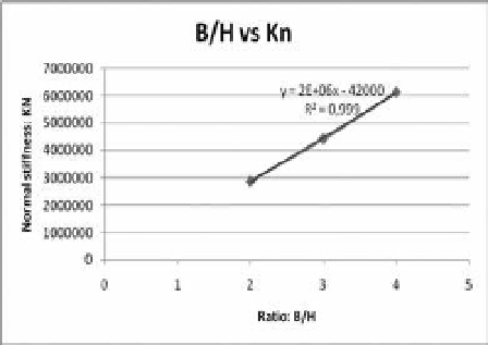
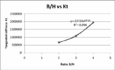
in addition, the normal stiffness (kn) and the
shear stiffness (kt) were calculated by dividing the
applied force against the obtained displacement.
The variation of the normal and shear stiffness
against the B/h ratio is shown in Figures 4 and 5.
in order to introduce the laws of behaviour in
the matrix system, the stiffness formulation for one
contact enounced by kishino (1989) and Tsutsumi
Σ F
X
= 0
(8)
Σ F
Y
= 0
(9)
Σ F
Z
= 0
(10)
where: {X, Y, Z} are the global axis. Using these
expressions for each particle in the macroporous
material it is obtained the following system:
[F] ⋅ {δ} = {i}
(11)
where:
[F] is the stiffness matrix of the system.
{δ} is the displacement vector of the particles
or spheres.
{i} is the vector that contains the load in the
three global axis {X, Y, Z}.
The procedure of calculus is the following:
Figure 4.
Relation between B/h ratio and normal
stiffness kn.
1. once the macroporous has been defined geo-
metrically, a normal stiffness (k
n
) and a shear
stiffness (k
t
) are assigned to each existing
contact (
Fig. 4-5
).
2. The local stiffness is projected to the global axis
to obtain the matrix [F], using the expressions
(5) to (10).
3. The vector {i} is built considering the forces
applied on the boundaries of the macroporous
material.
4. The matrix system of equations (11) is solved
and the displacements of each particle are
obtained. once the displacements are known,
Figure 5.
Relation between B/h ratio and the shear
stiffness kt.