Environmental Engineering Reference
In-Depth Information
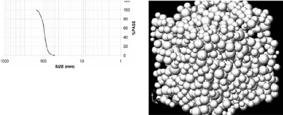
Figure 1. Grain size distribution for the particles that
formed the macroporous material.
Figure 3. example of a numerical macroporous mate-
rial of 1300 particles.
but a wall-beam model instead. By doing this,
it is obtained a joining tablet material in each
previously existing contact.
after all this process, a macroporous medium
is obtained. in Figures 2 and 3 it is shown some
examples of the macroporous created. The particles
are in white and the joining material in red. The
joining material is not in its real dimensions, it has
only been included to observe which particles are
in contact and which are not.
Figure 2. example of a numerical macroporous mate-
rial of 1300 particles.
3
eQUaTions oF The MoDel
in this point, the equations that command the
behavior of the macroporous material are shown.
in general, the macroporous can be under any kind
of load in each of its boundaries. But this research
is focused in modeling a consolidated triaxial test.
From the point of view of the strength, the
response of the medium is conditioned by the
joining material and its collapse. To model this
material, it has been assumed that a wall-beam,
similar to a tablet shaped material, under axial and
shear stresses is a good enough approximation.
The parameters considered for this material has
been the following ones:
probability of size is directly proportional to the
percentage retained by the size of each fraction,
according to the curve.
5. after this process, a cubic cell filled with
particles is obtained. These particles are in con-
tact but a joining material is filling those contacts,
keeping the particles joined and cohesioned. in
order to introduce this joining material a gap
is needed between the particles in contact. To
do this, a random uniform distribution between
two values was used to reduce the diameter of
the particles accordingly to it.
6. an elastic and breakable joining material was
inserted in the previously existing particle to
particle contacts. The joining material was
assimilated to square section prisms with a
section side (B) and a length (h) that was
determined in the fifth step. The B dimension
is randomly created using a random uniform
distribution between 2 and 6 times the length.
Doing this, a 2 to 6 B/h ratio is obtained. This is
necessary because a beam model is not wanted
E
= 600 MPa
(1)
V
= 0.2
(2)
σ
c
= 1 MPa
(3)
where: e is the Young´s modulus, ν is the Poisson's
ratio and σ
c
is the unconfined compressive
strength.