Graphics Reference
In-Depth Information
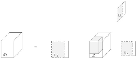
Figure 9.22
The
M
-mode SVD, illustrated for the case
M
=
3. (From [Vasilescu and Terzopoulos 04]
c
2004 ACM, Inc. Included here by permission.)
products,
D
=
Σ
×
1
U
1
×
2
U
2
.
(9.11)
Equation (9.11) can be readily generalized to express the
M
-mode SVD of an
order-
M
tensor
D
into the product of a tensor
Z
and
M
orthonormal matrices:
D
=
Z ×
1
U
1
×
2
U
2
···×
m
U
m
···×
M
U
M
.
(9.12)
The tensor
is the
core tensor
, which governs the interaction between the
M
matrices
U
m
and is analogous to
Z
in the ordinary matrix SVD; however, it is
no longer diagonal. The orthonormal matrices
U
m
are called
mode matrices
,and
are analogous to the orthonormal row and column matrices in the matrix SVD
of Equation (9.10). Figure 9.22 illustrates the
M
-mode SVD for the case
M
σ
=
3;
details of the computation can be found in the paper.
The data tensor created from typical BTF data is of third order, and the dimen-
sions are the number of texels
I
x
, the number of different illumination conditions
I
L
, and the number of different viewing directions
I
V
. The tensor modes corre-
spond to the variation in spatial pixels (texels), the variation in viewing direction,
and the variation in lighting direction. It is more convenient to call these modes by
name: “pixel mode” (or “texel mode”), “view mode,” and “illumination mode,”
respectively. The respective subscripts
x
,
V
,and
L
are used in place of integer
indices.
Because the two primary variables in the BTF are the viewing and illumination
directions, the data tensor is decomposed in terms of the illumination and view
modes:
D
=
T ×
L
U
L
×
V
U
V
.
(9.13)
The two mode matrices
U
L
and
U
V
contain the illumination and viewing varia-
tions, respectively. The
basis tensor
T
governs the interaction between the mode
matrices, and is defined as
T
=
Z ×
x
U
x
,
(9.14)