Modeling with Neural Networks: Principles and Model Design Methodology - Neural Networks: Methodology and Applications - page 125

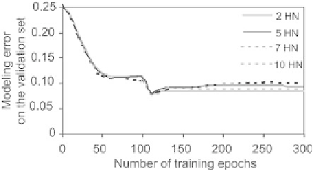
Fig. 2.12. Classification error on the validation set during training

The variation of the mean square error on a validation set of 300 examples,
as a function of the number of epochs, is shown on Fig. 2.12, for various num-
bers of hidden neurons. Clearly, deciding when training should be terminated
is di cult, because the error arises essentially from the examples that are
close to the boundary zone, which corresponds to a relatively small number
of points.
Therefore, that method is not very convenient, especially for classification.
Therefore, regularization methods that involve penalizing large parameters are
often preferred; it was proved [Sjoberg 1995] that early stopping is actually
equivalent to the introduction of a penalty term in the cost function.

2.5.4.2 Regularization by Weight Decay

Large values of the parameters, for instance of the parameters of the inputs
of hidden neurons, generate sharp variations of the sigmoids of the hidden
neurons: that is illustrated on Fig. 2.13, which shows function y = tanh( wx ),
for three different values of w . The output of the network, which is a linear
combination of the outputs of the hidden neurons, is therefore apt to exhibit
sharp variations as well. Regular outputs therefore require that the sigmoids be
in the vicinity of their linear zones, hence that the parameters not be too large.
We consider again the classification example of the previous section: Fig. 2.14
shows the variation of the module of the vector of parameters, during training,
for different architectures (2, 5, 7 and 10 hidden neurons). One observes that
the norm of the vector of parameters increases sharply during training, except
for the architecture with two hidden neurons: therefore, the sharp variations
of the output surface after training the network with ten hidden neurons, as
shown on Fig. 2.11, is not surprising.
Regularization by weight decay prevents the parameters from increasing
excessively, by minimizing, during training, a cost function J that is the sum
of the least squares cost function J (or of any other cost function, such as
cross entropy described in Chaps 1 and 6) and of a regularization term, pro-
portional to the squared norm of the vector of parameters: J ∗ = J + 2 i =1 w 2 ,

i