Information Technology Reference
In-Depth Information
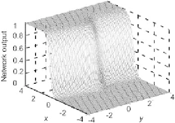
Fig. 2.10.
Posterior probability computed by a neural network with 2 hidden neu-
rons
p
X
(
x
| A
)Pr(
A
)
p
X
(
x
P
R
(
A
|
x
)=
B
)
,
|
A
)+
p
X
(
x
|
where
x
is the vector [
xy
]
T
,p
X
(
x
A
) is the distribution of the random vector
X
for the patterns of class
A
, and Pr(
A
) is the prior probability of class
A
.
The estimation provided by the neural network from the examples shown on
Fig. 2.8 should be as similar as possible to the surface shown on Fig. 2.9.
Training is performed with a set of 500 examples. A network with 2 hidden
neurons provides the probability estimate shown on Fig. 2.10; the estimate
provided by a neural network with 10 hidden neurons is shown on Fig. 2.11.
One observes that the result obtained with the network having 2 hidden
neurons is very close to the theoretical probability surface computed from
Bayes formula, whereas the surface provided with hidden neurons is almost
binary: in the zone where classes overlap, a very small variation of one of the
features generates a very sharp variation of the probability estimates. The 10-
hidden neuron network is over-specialized on the examples that are located
near the overlapping zone: it exhibits overfitting.
|
Fig. 2.11.
Posterior probability computed by a neural network with 10 hidden
neurons

Search WWH ::

Custom Search