Chemistry Reference
In-Depth Information
1.2
0.4
x
2
x
1
Negative profits
firm1
x
Positive profits
firm1
1.2
x
2
0
x
1
0
0.4
300
Time
370
(a)
(b)
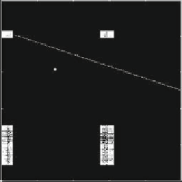
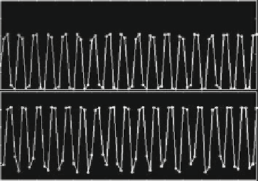
Fig. 3.5
Example 3.4; discrete time oligopoly with isoelastic demand and linear cost functions -
the duopoly case. The cost ratio
0:161.(
a
) A 4-cyclic chaotic attractor in the .x
1
;x
2
/
plane and dividing line between regions of positive and negative profits for firm 1. (
b
) Time series
of a portion of the chaotic attractor. Note how they are more regular than those in Fig. 3.4b
D
c
2
=c
1
D
profit line for firm 1 depicted in Fig. 3.5a indicates that the high-cost firm 1 would
make a loss after every fourth period with certainty, and potentially also makes a
loss after every third period. Consequently, given the regularity of the trajectories in
this situation and the possibility of losses following a regular pattern, it seems that
the assumption of naive expectations would be more plausible in the former case,
where the chaotic attractor extends over a larger portion of the phase space.
Let us now turn to the
semi-symmetric
case obtained by assuming c
2
D D
c
N
,
a
2
D D
a
N
, L
2
D D
L
N
and x
2
.0/
D D
x
N
.0/. This particular situa-
tion, which has been already studied in Example 3.3, allows us to get some insight
into the effects of increasing the number of competitors. As we have seen already in
the previous chapters, if the firms partially adjust their production quantities towards
the best replies, then the decisions made by firm 1 and the identical firms 2;:::;N
are captured by the two-dimensional dynamical system
x
1
.t
C
1/
D
.1
a
1
/x
1
.t/
C
a
1
R
1
..N
1/x
2
/;
x
2
.t
C
1/
D
.1
a
2
/x
2
.t/
C
a
2
R
2
.x
1
C
.N
2/x
2
/:
T
W
Assuming an interior equilibrium, it is given by
.N
1/c
2
.N
2/c
1
c
1
C
.N
1/c
2
;
.N
1/A
c
1
C
.N
1/c
2
x
1
D
c
1
c
1
C
.N
1/c
2
.N
1/A
c
1
C
.N
1/c
2
x
2
D
:::
D
x
N
D


Search WWH ::

Custom Search