General Oligopolies - Nonlinear Oligopolies: Stability and Bifurcations - page 113

0.4

1.2

x 1

x 2

Negative profits
firm1

1.2

Positive profits
firm1

x 2

0

300 370

x 1

0 0.4

Time

(a) (b)

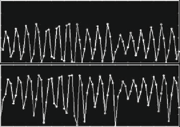
Fig. 3.4 Example 3.4; discrete time oligopoly with isoelastic demand and linear cost functions -
the duopoly case. The cost ratio 0:16.( a ) The chaotic attractor in the .x 1 ;x 2 / plane

and the dividing line between regions of negative and positive profits for firm 1. ( b ) Time series of
a portion of the chaotic attractor

D c 2 =c 1 D

loses stability via a pe riod do ub ling bifurcation. For values of the cost ratio outside

the interval .3 2 p 2;3 C 2 p 2/ the asymptotic dynamics may converge to periodic
cycles or even exhibit chaotic motion around the Nash equilibrium. A numerically
computed chaotic trajectory is shown in Fig. 3.4, obtained for A D 1, a 1 D a 2 D 1,
c 1 D 1, c 2 D 0:16. It can be noticed that the chaotic area is quite large, hence
we expect no correlations between x 1 .t/ and x 2 .t/, in the sense that high values
of x 1 .t/ are associated either with high or with low values of x 2 .t/ in the same
time period; see Fig. 3.4b, where a portion of the chaotic trajectory of Fig. 3.4a is
represented for the time periods t 2 Œ300;370. Note that the profits for the firms are
non-negative only if x 1 C x 2 A=c k ;k D 1;2. In Fig. 3.4a we depict the line of
zero profits for firm 1, which is represented by the equation x 1 C x 2 D A=c 1 D 1.
Notice that the zero profit line of firm 2, x 1 C x 2 D 6:25, is outside the area shown in
the figure. This indicates that the profits for the low-cost firm 2 are always positive,
whereas firm 1 makes a loss in some periods along any trajectory which describes
the long-run dynamics. The latter point becomes even more obvious if we consider
other kinds of long-run dynamics for the duopoly with best reply dynamics. For
example, let c 2 D 0:161, with all other parameter values as before. The cost ratio
is now outside the stability region, and the disequilibrium dynamics in this case are
described by a 4-cyclic chaotic attractor 1 (see Fig. 3.5 2 ). Of course, even if in this
case chaotic dynamics are observed, the time series are much more regular, since
they are characterized by a quasi-cyclic behavior (Fig. 3.5b). Furthermore, the zero

1 An n-cyclic chaotic attractor consists of n separate pieces that are visited cyclically in a given
order.
2 The particular “rectangular shape” of the attractors shown in Figs. 3.4 and 3.5 is related to the
particular structure of the map in the case of best reply dynamics, see for example, Bischi et al.
(2000b) and Agliari et al. (2002a)