General Oligopolies - Nonlinear Oligopolies: Stability and Bifurcations - page 115

and it is locally asymptotically stable if

4a 1 .N 1/ C a 1 a 2 .1 C .N 1// 2 C 2a 2 . 2 C N.1 C N// < 0

8. 2 C a 1 /.N 1/ C a 1 a 2 .1 C .N 1// 2

C 4a 2 . 2 C N.1 C N// > 0;
(3.15)

where D c 2 =c 1 denotes the cost ratio between firms (see Example 3.3; recall that
the other stability condition derived there is always fulfilled). For given adjustment
coefficients and unit costs, these conditions tell us for which number of firms the
equilibrium becomes unstable. Consider for example A D 16, a 1 D 0:4, a 2 D 0:3,
c 1 D 5, c 2 D 6, L 1 D L 2 D 2. Then it is easy to see that the first condition holds
always for N>2, so we do not consider it in the following analysis. The second
inequality becomes 88N 2 C 1246.N 1/>0, and it holds as long as the number

of firms N 13. So in these cases the equilibrium is stable. For N D 14 this inequal-
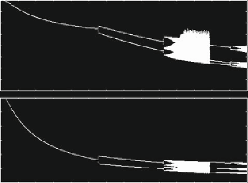
ity is violated, showing that the equilibrium becomes unstable. Figure 3.6 shows a
bifurcation diagram for N in the range Œ2;30. As expected, the Nash equilibrium
x is stable as long as the number of competitors is less than 13, and then it loses
stability through a period doubling bifurcation. For even higher values of N other
bifurcations occur leading to more complicated kinds of asymptotic behavior. Since
more detailed results can be easily derived on the basis of a standard local stability
analysis, we now turn to the more interesting investigation of the global properties
of our model.
In order to explain what kind of bifurcations and global dynamic properties are
involved in the qualitative changes of the dynamics observed in Fig. 3.6, we study
the properties of the piecewise smooth map T . We first divide the strategy space

0.8

x 1

0

0.6

x 2

0

2 6 10 14 18 22 26 30

N

Fig. 3.6 Example 3.4; discrete time oligopoly with isoelastic demand and linear cost functions -
the semi-symmetric case. Bifurcation diagrams of outputs x 1 ;x 2 with respect to the number of
firms