Civil Engineering Reference
In-Depth Information
In (
5
), f
ij
is the frequency of being in state i and transit to state j. The transition
matrix P is computed just by counting each state frequency and dividing that by
the total amount of transitions (Ching and Ng
2005
).
3.5 Model Validation
The validation process takes advantage of the stationarity of the ECM stochastic
model. This implies that its statistical characteristics do not change over time. That
is, the provided time series varies over time; however, its characteristics such as
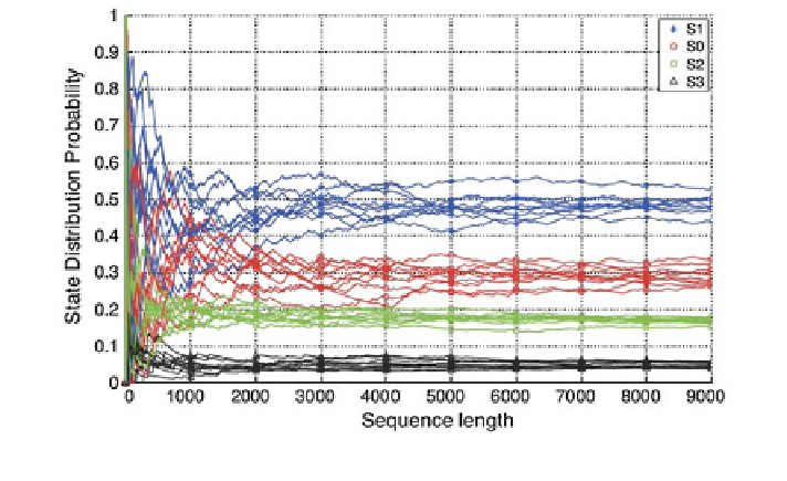
mean and variance converge to constant values. The cumulative state distribution
over a finite horizon for a MC similar to the one in Fig.
7
a is depicted in Fig.
8
.
Since the model is stochastic, the generated sequences in Fig.
7
b, also referred as
time series or paths, are different. However, with this model structure, the state
probability distribution converges to a stationary distribution also referred as
steady state distribution (Pollard
1984
). The steady-state distribution is a charac-
teristic of the model and not of the generated sequence. Generally, there are two
ways of determining the steady-state distribution, either by simulation or by
analytically. The simulation method consists in generating a sequence with the
model over a sufficient large period. Next, the generated sequence is analysed, and
the state distribution is computed. The problem is to define how large should the
period be for the different models. The analytical method uses the time-homo-
geneous property of the MC as follows:
Fig. 8
Simulation of a Markov chain with 4 states over different initial conditions