Information Technology Reference
In-Depth Information
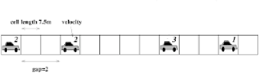
Fig. 1.
Part of a road in the Nagel-Schreckenberg model
x
n
is the position of the
n
th car and
v
n
∈{
1
,
2
,... ,v
max
}
its velocity.
v
max
denotes the maximum velocity and
d
n
is the number of empty cells (gap) in
front of car
n
. One time-step corresponds to 1s in real time.
The first two rules (step 1 and 2) describe a somehow optimal driving strat-
egy: the driver accelerates if the vehicle has not reached the maximum velocity
v
max
and brakes to avoid accidents, which are explicitly excluded. However,
drivers do not react in this optimal way: they vary their speed without any
obvious reason, reflected by the
braking noise p
(step 3). It mimics the com-
plex interactions between the vehicles and is also responsible for spontaneous
formation of jams.
2.2 More Realistic Cellular Automaton Model
The first model implemented in our simulator was the basic Nagel-Schreckenberg
cellular automaton model, but a more realistic tra
c flow is obtained by using
smaller cells and by extending it with
velocity dependent randomization
,
antici-
pation
, and
brake lights
.
Smaller cells allow a more realistic acceleration and more speed bins. We are
currently using a cell size of 1
.
5m, which corresponds to speed bins of 5
.
4km
/
h
and an acceleration of 1
.
5m
/
s
2
(0
−
100km
/
h in 19s). A vehicle occupies 2
−
5 con-
sequent cells. By using velocity dependent randomization [7] meta-stable tra
c
flows are modeled by the simulator, a phenomenon observed in empirical studies
of real tra
c flows [12,13,14]. By including anticipation and brake lights [8,10] in
the modeling, the cars not solely determine their velocity in dependency of the
distance to the next car in front, but also take regard to its speed and whether
it is reducing the speed or not. These modifications of the Nagel-Schreckenberg
model imply that we have to add some new parameters to the model.
When the simulation algorithm decides if a car
n
should brake or not it does
not only look how far away the next car
m
in front is, but makes an estimate of
how far the car
m
will move during this time-step (anticipation). Note, that the
moves are done in parallel, so the model remains free of collision. This leads to
the effective gap
d
e
n,m
(
t
):=
d
n,m
(
t
) + max(
v
mi
m
(
t
)
− d
S
,
0)
seen by car
n
at time
t
. In this formula
d
n,m
(
t
) is the number of free cells between
the front of the car
n
and the back of the car
m
,
d
S
is a safety distance, set equal
to 6 cells (9m) in our model, and