Environmental Engineering Reference
In-Depth Information
1.0
3.4 White noises and Brownian motions
The construction of a time series can be modelled with a
Gaussian white noise
. This is an uncorrelated set of values
obtained from a Gaussian distribution. The Gaussian
white noise is the cla
s
sic example of a stationary time
series, with a mean
x
and variance
Power-law
Distribution
Gaussian
Distribution
f
(
x
)
0.5
x
of the values
specified. A typical example is given in Figure 3.4a. For
each of the
n
σ
, 512 values given, a random
number in the range 0
.
0
≤
F
(
x
n
)
≤
1
.
0 is chosen. We
choose the value of 512 (i.e. 2
9
) for convenience in using
the Fourier Transform introduced below (Section 3.5.3).
The cdf for the Gaussian distribution in Figure 3.2 is
then used to convert each
F
(
x
n
) value to corresponding
values of
x
n
, by projection down to the horizontal axis.
Uncorrelated Gaussian time series can also be created
by many computer programs (Press
et al
., 1994), using
'random' functions, but care must be taken that the time
series are truly uncorrelated and that the frequency-size
distribution is specified (an example where these issues
are discussed in the context of landslide time series is
given by Witt
et al
., 2010).
The classic example of a non-stationary time series is a
Brownian motion
(Wang and Uhlenbeck, 1945), which is
obtained by summing a Gaussian white noise with zero
mean. The motion of a molecule in a gas is a Brownian
motion (Einstein, 1956). The running sum,
x
n
,ina
Brownian motion time series is given, on average over
many simulations, by:
=
1, 2, 3,
...
0.0
0
1
2
3
4
5
6
7
8
x
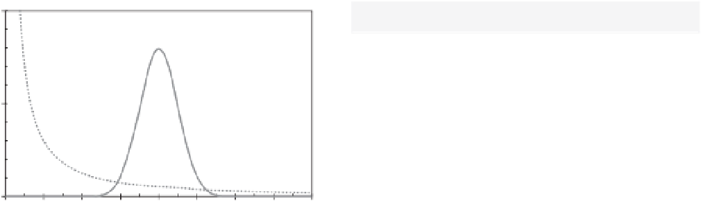
Figure 3.3
The noncumulative probability
f
(
x
) is given as a
function of
x
for a symmetrical 'thin-tailed' Gaussian
distribution and a 'fat-tailed' nonsymmetrical power-law
distribution. The Gaussian (mean 4.0, standard deviation 0.5)
has tails (the very smallest or very largest sizes) that fall off as an
exponential (Equation 3.2). This contrasts with the inverse
power-law distribution,
f
(
x
)
x
−
C
, where the exponent here is
∼
C
2; the tail of the power-law distribution here falls off
much more slowly than the right-hand Gaussian tail. Many
environmental datasets are strongly non-Gaussian (e.g.,
earthquakes, wildfires), following power-law or other fat-tailed
distributions.
=
1
.
tail of the Gaussian distribution is said to be
'thin tailed'
,
whereas the power-law tail of the Pareto distribution is
fat (or heavy) tailed
. An important aspect of these fat-
tailed distributions is that, if natural phenomena follow
a fat-tail versus a thin-tail distribution, the probability
of catastrophic events is much greater. For instance, the
preferred distributions for the occurrence of severe wild-
fires, floods, and other natural hazards are 'thin-tailed'
in some countries and 'fat-tailed' in others, resulting in
very diverging views of the risk involved for those hazards
(Malamud, 2004).
In this section, we have discussed the Gaussian (nor-
mal) and the Pareto (power-law) distributions. There are
many other kinds of statistical distributions, the most
common of which may be divided into four families: the
normal family (normal, log-normal, log-normal type 3),
the general extreme-value (GEV) family (GEV, Gumbel,
log-Gumbel, Weibull, Cauchy), the Pearson type 3 family
(Pearson type 3, log-Pearson type 3), and the generalized
Pareto distribution. Stedinger
et al
. (1993) provide an
excellent discussion and review of these different distri-
butions. In the next section, in the context of stationarity
and time series, we will also discuss briefly the log-normal
distribution.
n
i
=
1
ε
i
x
n
=
(3.4)
wher
e
ε
i
are the randomvalues in a white-noise time series
with
x
0. The white noise illustrated in Figure 3.4a has
been summed to give the Brownian motion illustrated in
Figure 3.4b. The variance of a Brownian motion, after
n
values, is given by
=
σ
ε
n
)
0
.
5
σ
=
[
x
n
]
(
(3.5)
where
σ
ε
is the standard deviation of the white-noise
sequence. In Figure 3.4c, we show the superposition of
twelve Brownianmotions. The relation fromEquation 3.5
is included in Figure 3.4c, as the solid line parabola,
illustrating the drift of Brownian motions. Brownian
motions have no origin defined, successive increments
are random, and they are an important model for time
series, which we will discuss more in depth in Section 3.5.


Search WWH ::

Custom Search