Time Series: Analysis and Modelling - Environmental Modelling: Finding Simplicity in Complexity - page 32

4

2

0

x n

− 2

− 4

0 128 256 384 512

n

(a)

40

20

0

x n

− 20

− 40

0 128 256 384 512

n

(b)

40

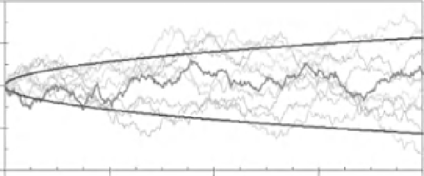
Figure 3.4 White noise and Brownian
motions. (a) An example of a Gaussian
white noise. Successive values are chosen
randomly from a Gaussian distribution
( E quation 3.2, Figure 3.2) with zero mean
( x = 0 . 0) and unit variance ( σ

20

0

x n

x = 1 . 0).
Adjacent values are not correlated. (b) The
white noise in (a) is summed using
Equation 3.4 to give a Brownian motion.
(c) Twelve examples of Brownian motions
are superimposed, each constructed from a
white noise. The envelope (solid parabolic
line) gives the standard deviation after n
steps (Equation 3.5).

− 20

− 40

0 128 256 384 512

n

(c)

We have shown how an uncorrelated time series can
be created with a Gaussian distribution of values. How-
ever, the Gaussian distribution has limitations, including
the fact that the distribution is symmetric and values
are specified over the range −∞ < x n < ∞ . Many time
series have frequency-size distributions that are heavily
asymmetric and/or are restricted to only positive values.

All five real-world time series given in Figure 3.1 have
positive values only, with just two of the examples show-
ing (some) symmetry in the frequency-size distributions.
There are many other statistical distributions used to
model time series, with just one example of a widely
used one for positive values (and asymmetry) being the
log-normal distribution.