Environmental Engineering Reference
In-Depth Information
n
,
N
, with
n
the time index, successive
x
n
separated by a sampling interval
=
1, 2, 3,
...
1.0
(including units of
time), and
N
the number of observed data points. The
length of the time series is
T
δ
F
(
x
)
=
δ
. Here, we focus our
attentionondiscrete time series with values equally spaced
in time, recognizing that time series that are unequally
sampled or with few non-zero values unequally spaced,
also are com
m
on.
The
mean x
and
variance
N
0.5
f
(
x
)
x
of the time series values
x
n
taken over
N
values are given by:
σ
0.0
−
4
−
3
−
2
−
10
1234
N
N
1
N
1
x
x
)
2
x
(no units)
x
=
x
n
,
σ
=
(
x
n
−
(3.1)
N
−
1
n
=
1
n
=
1
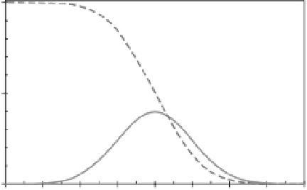
Figure 3.2
The probability distribution function
f
(
x
) (solid
line) and the cumulative distribution function
F
(
x
) (dashed
line) for the standa
rd
form of the Gaussian (normal)
distribution, mean
x
where
σ
x
is the standard deviation.
The discrete values
x
n
can be characterized by a con-
tinuous
frequency-size distribution f
(
x
), i.e., the relative
number of large, medium, and small values that are in the
time series. A widely applicable frequency-size distribu-
tion frequently used to model time series is the
Gaussian
(normal) distribution
. The probability density function
(pdf) for this distribution takes the form:
=
.
σ
x
=
.
0
0 and standard deviation
1
0,
from Equations 3.2 and 3.3.
the
k
th
moment is determined by taking a value in a
distribution, subtracting the mean, raising this to the
k
th
power, doing this again for all other values in the
distribution, summing the results, and properly normal-
izing. For some time series, higher moments can also
be specified, such as the
skewness
(third-order moment),
kurtosis
(fourth-order moment), and so on, to reflect the
lack of symmetry or spikiness of the distribution. For
the Gaussian distribution, these higher moments are zero
because of the symmetry and shape of the distribution. A
stationary time series
is one in which a given moment, if it
exists, is independent of the length of the interval within
a time series considered. If a given moment increases or
decreases as a function of the interval length, the time
series is
non-stationary. Weak stationarity
is where the
mean and the variance are approximately independent of
the length of the interval considered. In weak stationarity,
highermoments of the frequency-size distribution are not
considered.
Strong (strict) stationarity
is where the mean
and the variance, if they exist, do not change at all as a
function of length of the interval considered. Stationar-
ity will be discussed throughout this chapter, along with
examples, and will be assumed to be weak stationarity
unless indicated otherwise.
Another frequency-size distribution of interest for
modelling time series is the
Pareto distribution
.The
important aspect of this distribution is the frequency
of occurrence of large values decays as a
power law
of
the values. This behaviour contrasts with the Gaussian
distribution, which decays as an
exponential
of large val-
ues. This contrast is shown in Figure 3.3. The exponential
σ
x
exp
−
x
)
2
1
(
x
f
(
x
)
=
−
(3.2)
π
)
0
.
5
σ
x
(2
2
where
x
and
σ
x
are the mean and standard deviation of
the probability distribution and 'exp' is the exponential
function. The probability that the value
x
lies in the
range (
x
1
2
1
2
x
.In
addition to characterizing the
noncumulative probability
of a given value occurring at a given size (the pdf), one
can also characterize the
cumulative probability
of a value
occurring greater than or equal to (or less than or equal
to) a given size. A
cumulative distribution function
(cdf) is
obtained from the probability distribution (pdf) function
by the integration:
−
x
)to(
x
+
x
)isgivenby
f
(
x
)
∞
F
(
x
)
=
f
(
u
)d
u
(3.3)
x
In this case
F
(
x
) is the probability that a value
u
in the
distribution lies between
x
and infinity. The pdf and cdf
for the Gaussia
n
distribution are given in Figure 3.2 taking
a mean value
x
=
0 and a standard deviation
σ
x
=
1
.
0
(called the standard Gaussian distribution).
The Gaussian frequency-size distribution is a
symmet-
r
ic distribution
that is completely specified by its
m
ean
x
and its standard deviation
σ
x
. The quantities
x
and
x
are the first- and second-order statistical
moments
of
any distribution of time-series values. Different moments
described the shape of a statistical distribution, where
σ


Search WWH ::

Custom Search