Time Series: Analysis and Modelling - Environmental Modelling: Finding Simplicity in Complexity - page 29

1000

500

0

1945 1950 1955 1960 1965 1970 1975 1980 1985

Year

(c)

2000

1500

1000

500

0

0 500 1000 1500 2000

Date

(d)

30

20

10

0

Jan Feb Mar Apr May Jun Jul Aug Sep Oct Nov Dec

Date

(e)

Figure 3.1 ( Continued )

measured at the Mauna Loa Observatory, Hawaii, are
given as a function of time for January 1980 to July
2010. The main features of this time series are an annual
periodicity superimposed on a near-linear trend over
the length of record. The annual periodicity is attributed
to summer vegetation in the northern hemisphere
extracting CO 2 from the atmosphere. The near-linear
trend is attributed to anthropogenic CO 2 emissions.
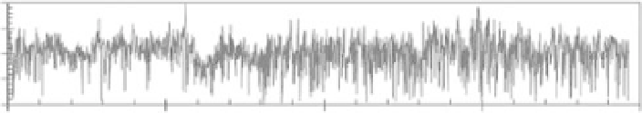
In Figure 3.1b, the numbers of earthquakes worldwide
with moment magnitude M W ≥

This contrasts with Figure 3.1b, where the frequency-size
distribution of values is quasi-symmetric with respect to
the mean, with approximately the same number of 'large'
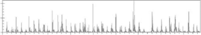
values as 'small' ones. In Figure 3.1d, the standardized
tree-ring-growth indexes for the bristlecone pine atWhite
Mountain, California are given for 1962 years. The dis-
tribution is also relatively symmetric with respect to the
mean, but there are clear correlations in the data, intervals
of low values and intervals of high values. In Figure 3.1e,
total daily precipitation in London, UK, is given for the
calendar year 2009. There are many days when there
was no precipitation, leading to discontinuities in the
data set, where the positive values are unequally spaced
in time. This type of data can be particularly difficult
to model.

6 in successive 14-day
intervals are given as a function of time for 1977 to 2007.
There are no apparent trends or periodicities in this time
series. Successive values appear to be either uncorrelated
or very weakly correlated. This pattern would be expected
to be the case for global seismicity, with the exception of
aftershocks.
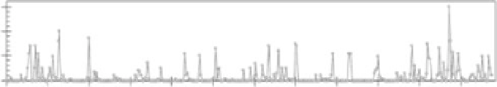
In Figure 3.1c, the daily mean discharge on the Sacra-
mento River near Delta, California is given as a function
of time for 1945 to 1988. A strong annual component is
clearly illustrated. Also, the frequency-size distribution of
values is strongly asymmetric, i.e., the large extreme val-
ues (the floods) stand out relative to the mean of the data.

3.3 Frequency-size distribution of values
in a time series

Values in a time series can be continuous in time, x ( t ),
or they can be given at a discrete set of times, x n ,