Information Technology Reference
In-Depth Information
−
0.1
r
−
8
−
10
0
g
−
6
RGF
7
−
4
q
−
2
6
SLF
u
v
0.1
c
h
6
0
m
p
j
5
5
2
4
2
i
3
1
f
0
0.2
4
b
n
−
1
6
−
2
a
3
−
3
8
k
d
10
2
0.3
w
12
s
e
SPR
1
14
t
0.4
PLF
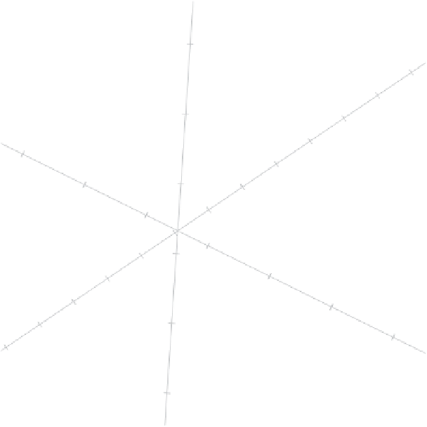
Figure 2.23
Illustration of vector-sum interpolation. The vertices of the blue quadrangle
area give the values of the four variables to be interpolated. The end of the black arrow
marks the centroid of the four vertices. The length of the red arrow is four (
p
)
times the
length of the black arrow and indicates the position of the interpolated point.
The
r
elements of the column vector
b
r
may be taken as a point which, when joined
to the origin, gives the direction of a new axis which can be calibrated and used in the
usual way.
In (2.18) we have used the notation
V
r
introduced in Section 2.2 to denote the first
r
columns of the orthogonal matrix
V
, thus avoiding complications with inverting singular
matrices. We may simplify the expression for
b
r
by using the notation for the rank-
r
approximation
U
r
r
V
r
to
X
=
U
V
.Then
V
r
X
XV
r
=
2
r
and
XV
r
=
U
r
r
, giving
b
r
=
−
1
U
r
x
∗
.
(2.19)
r
In terms of the
J
-notation (2.19) may be rewritten as
b
r
0
:
p
×
1
=
J
−
1
U
x
∗
=
Jb
,
(2.20)
showing that different settings of
r
in
J
give the regression for any number of dimensions
used in the PCA approximation, including the full
p
-dimensional solution, when
J
=
I