Information Technology Reference
In-Depth Information
−
0.1
r
10
−
−
8
0
g
6
−
RGF
7
−
4
q
−
2
6
SLF
u
v
0.1
h
0
6
j
5
5
c
2
m
4
p
2
3
i
1
f
4
0
0.2
4
b
n
−
1
6
−
2
a
8
3
−
3
d
10
k
2
0.3
w
12
s
e
1
SPR
14
t
0.4
PLF
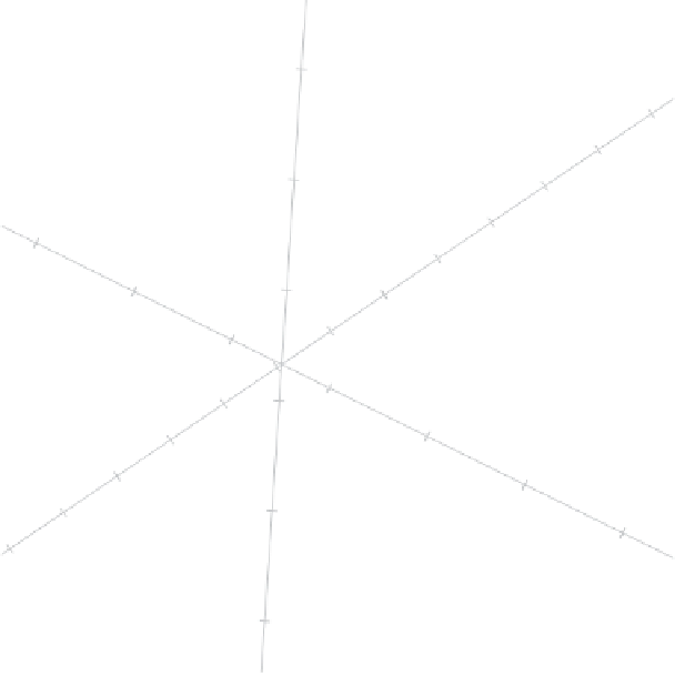
Figure 2.22
Interpolation biplot of the scaled aircraft data in Table 2.2.
The biplots constructed in this topic will be fitted with prediction biplot axes unless
stated otherwise. This is because it is intuitive for anyone analysing a plot to read off
values for the variables on the axes. In general, the interpolation can be taken care
of algebraically with a computer program, as is illustrated in the functions contained in
UBbipl
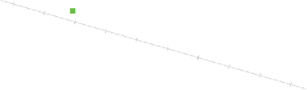
. As an example, we show in Figure 2.27 the result of interpolating the new point
with values
SPR
=
8,
RGF
=
4,
PLF
=
0
.
3and
SLF
=
3 using the algebraic formula
for interpolation by specifying the argument
X.new.samples = matrix(c(8,4,0.3,
3), nrow = 1))
.
2.7 Adding new variables: the regression method
We have seen above how to add new samples to a PCA. Suppose now that we wish to
add a new variable available in a centred column vector
x
∗
:
n
1. We may add
x
∗
to our
PCA by using a regression method that assumes that
x
∗
is approximately a linear function
x
∗
=
×
XV
r
b
r
of the points
XV
r
. This is a multiple regression problem with solution
b
r
:
r
×
1
=
(
V
r
X
XV
r
)
−
1
V
r
X
x
∗
.
(2.18)